
Chapter 1. Introduction to Geology
Adapted by Karla Panchuk from Physical Geology by Steven Earle
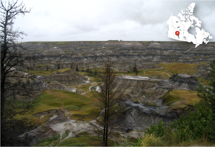
Learning Objectives
After reading this chapter and answering the review questions at the end, you should be able to:
- Explain what geology is, and why we study Earth.
- Describe the kinds of work that geologists do.
- Explain what is meant by geological time.
- Explain how the principle of uniformitarianism allows us to translate observations about Earth today into knowledge about how Earth worked in the past.
- Summarize the main idea behind the theory plate tectonics.
1.1 What Is Geology?
Geologists study Earth — its interior and its exterior surface, the rocks and other materials around us, and the processes that formed those materials. They study the changes that have occurred over the vast time-span of Earth’s history, and changes that might take place in the near future.
Geology is a science, meaning that geological questions are investigated with deductive reasoning and scientific methodology. Geology is arguably the most interdisciplinary of all of the sciences because geologists must understand and apply other sciences, including physics, chemistry, biology, mathematics, astronomy, and more.
An aspect of geology that is unlike most of the other sciences is the role played by time — deep time — billions of years of it. When geologists study the evidence around them, they are often observing the results of are observing the results of events that took place thousands, millions, and even billions of years in the past, and which may still be ongoing. Many geological processes happen at incredibly slow rates — millimetres per year to centimetres per year — but because of the amount of time available, tiny changes can result in expansive oceans forming, or entire mountain ranges being worn away.
Geology on a Grand Scale in the Canadian Rocky Mountains
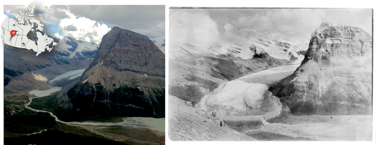
The peak on the right of the photographs in Figure 11.2 is Rearguard Mountain, which is a few kilometres northeast of Mount Robson. Mount Robson is the tallest peak in the Canadian Rockies, at 3,954 m. The large glacier in the middle of the photo is the Robson Glacier. The river flowing from Robson Glacier drains into Berg Lake in the bottom right.
Many geological features are shown here. The rocks that these mountains are made of formed in ocean water over 500 million years ago. A few hundred million years later, the rocks were pushed east for tens to hundreds of kilometres, and thousands of meters upward in a great collision between Earth’s tectonic plates.
Over the past two million years this area, like most of the rest of Canada, has been repeatedly covered by glaciers that scoured away rocks to form the valley to the left of Rearguard Mountain. The Robson Glacier itself is now only a fraction of its size during the Little Ice Age of the 15th to 18th centuries. And, like almost all other glaciers on Earth, it is now receding even more rapidly because of climate change. Figure 11.2 (right) taken around 1908 by the Canadian geologist and artist Arthur Philemon Coleman, gives an indication of how much the glacier has receded in the last hundred years.
Geology is about understanding the evolution of Earth through time. It is about discovering resources such as metals and energy, and minimizing the environmental implications of our use of resources. It is about learning to mitigate the hazards of earthquakes, volcanic eruptions, and slope failures. All of these aspects of geology, and many more, are covered in this textbook.
References
Victoria University Library (2009) A. P. Coleman Exhibition. Retrieved 25 August 2017. Visit the website
1.2 Why Study Earth?
Why? Because Earth is our home — our only home for the foreseeable future — and in order to ensure that it continues to be a great place to live, we need to understand how it works. Another answer is that some of us can’t help but study it because it’s fascinating. But there is more to it than that.
- We can study rocks and the fossils they contain to understand the evolution of our environment and the life within it.
- We can learn to minimize our risks from earthquakes, volcanoes, slope failures, and damaging storms.
- We can learn how and why Earth’s climate changed in the past, and use that knowledge to understand both natural and human-caused climate change.
- We rely on Earth for resources such as soil, water, metals, industrial minerals, and energy, and we need to know how to find these resources and exploit them sustainably.
- We can recognize how human activities have altered the environment, and learn how to prevent and sometimes repair the damage.
- We can use knowledge of Earth to understand other planets in our solar system, and those around distant stars.
The Importance of Geological Studies for Minimizing Risks to the Public
Figure 1.3 shows a slope failure that took place in January 2005 in the Riverside Drive area of North Vancouver. The steep bank beneath the house shown gave way, and a slurry of mud and sand flowed down. It destroyed another house below, and killed one person. The slope failure happened after a heavy rainfall, which is a common occurrence in southwestern B.C. in the winter.
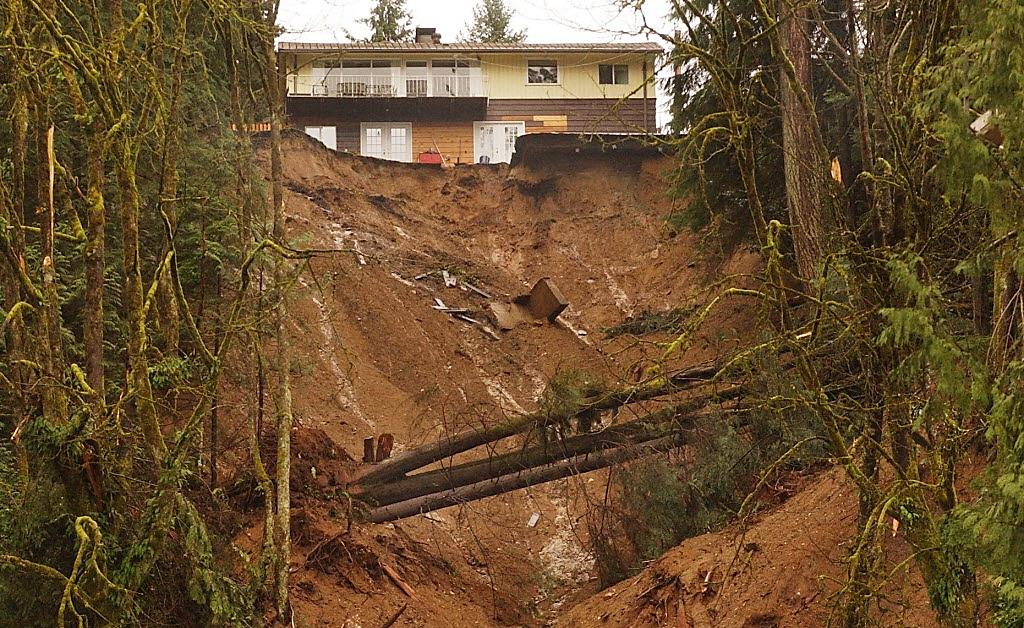
A geological report written in 1980 warned the District of North Vancouver that the area was prone to slope failure, and that steps should be taken to minimize the risk to residents. Unfortunately, not enough was done in the intervening 25 years to prevent a tragedy.
1.3 What Do Geologists Do?
Geologists do a lot of different things. Many of the jobs are the things you would expect. Geologists work in the resource industry, including mineral exploration and mining, and exploring for and extracting sources of energy. They do hazard assessment and mitigation (e.g., assessment of risks from slope failures, earthquakes, and volcanic eruptions). They study the nature of the subsurface for construction projects such as highways, tunnels, and bridges. They use information about the subsurface for water supply planning, development, and management; and to decide how best to contain contaminants from waste.
Geologists also do the research that makes practical applications of geology possible. Some geologists spend their summers trekking through the wilderness to make maps of the rocks in a particular location, and collect clues about the geological processes that occurred there. Some geologists work in laboratories analyzing the chemical and physical properties of rocks to understand how the rocks will behave when forces act on them, or when water flows through them. Some geologists specialize in inventing ways to use complex instruments to make these measurements. Geologists study fossils to understand ancient animals and environments, and go to extreme environments to understand how life might have originated on Earth. Some geologists help NASA understand the data they receive from objects in space.
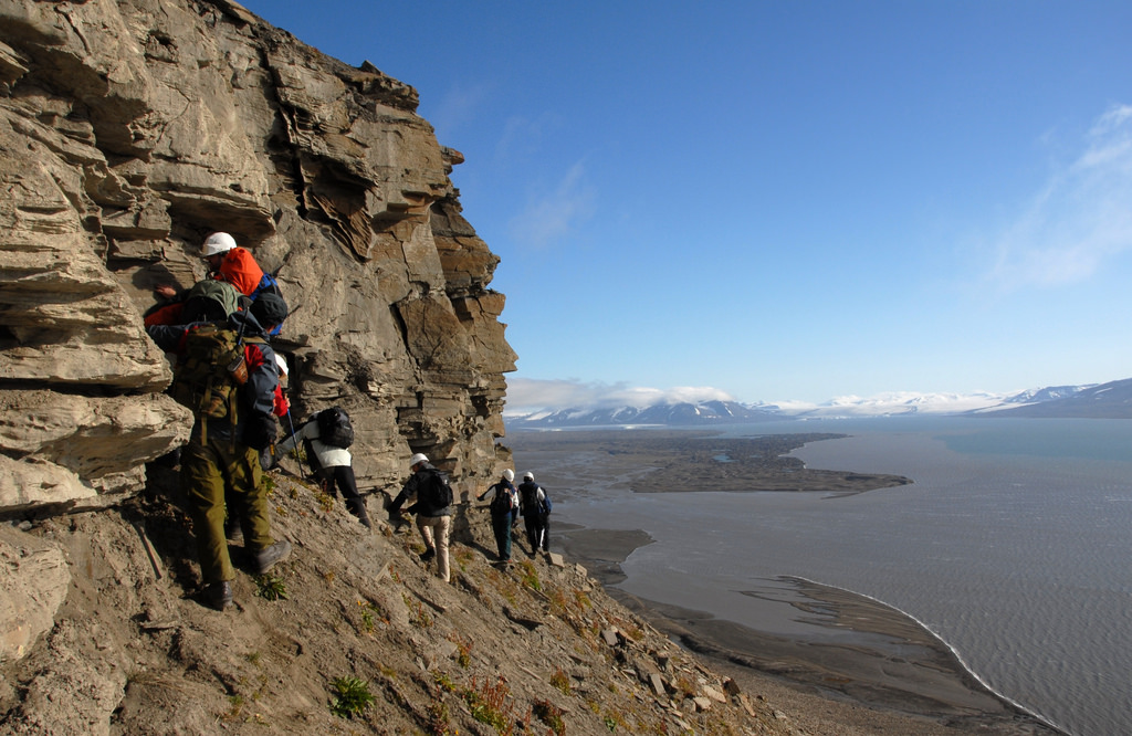
Geological work can be done indoors in offices and labs, but some people are attracted to geology because they like to be outdoors. Many geological opportunities involve fieldwork in places that are as amazing to see as they are interesting to study. Sometimes these are locations where few people have ever set foot, and where few ever will again.
1.4 We Study Earth Using the Scientific Method
There is no single method of inquiry that is specifically the scientific method. Furthermore, scientific inquiry is not necessarily different from serious research in other disciplines. The key features of serious inquiry are the following:
- Creation of a hypothesis. This is a tentative idea about how to explain a set of observations.
- Test the hypothesis. A hypothesis can be used to make predictions, and experiments can be run to see if those predictions are correct.
An Example of the Scientific Method at Work
Consider a field trip to the stream shown in Figure 1.5. Notice that the rocks in and along the stream are rounded off rather than having sharp edges. We might hypothesize that the rocks were rounded because as the stream carried them, they crashed into each other and pieces broke off.

If the hypothesis is correct, then the further we go downstream, the rounder and smaller the rocks should be. Going upstream we should find that the rocks are more angular and larger. If we were patient we could also test the hypothesis by marking specific rocks and then checking back to see if those rocks have become smaller and more rounded as they moved downstream.
If the predictions turn out to be correct, we must still be careful about how much certainty to attach to our hypothesis. Although our hypothesis might seem to us to be the only reasonable explanation, someone could argue that we have the mechanism wrong, and the rocks weren’t rounded by bumping into each other. If our experiment didn’t specifically check for the mechanism (e.g., by looking to see if chips fall off the rocks and the rocks are made smoother) then we would have to acknowledge the possibility. We needn’t abandon the hypothesis as a useful tool for making predictions, but it is necessary to be open to the possibility that other things might be going on. If someone demonstrates conclusively that our hypothesis is wrong, then we have to discard the hypothesis and come up with a better one.
A good hypothesis is testable. Someone might argue that an extraterrestrial organization creates rounded rocks and places them in streams when nobody is looking. There is no practical way to test this hypothesis to confirm it, and there is no way to prove it false. Even if we never see aliens at work, we still can’t say they haven’t been, because according to the hypothesis they only work when people aren’t looking. Compare this to our original hypothesis which allows us to make testable predictions such as rocks getting smaller and rounder downstream. Our original hypothesis gives us a way to see how realistic it is, whereas the alien hypothesis gives us no way to know if it makes sense or not.
Theories and Laws
Two other terms appear in discussions of the scientific method: theory and law. A theory starts out as a hypothesis, but over a long period of time and a great many tests, it has never come up short. That doesn’t mean it never will, but the odds of that are very unlikely given our present (and conceivable future) state of knowledge. You may have heard someone dismiss an idea by saying it is “just a theory,” but they are using the term incorrectly if they mean to say it’s a wild and unproven guess.
A law is a description of a phenomenon rather than an explanation of it. For example, you could do thousands of tests by dropping an object with known mass and measuring its acceleration and the force with which it hits the ground. Again and again your results will yield the formula force = mass x acceleration. However, that doesn’t mean you know what is responsible for the force accelerating it toward the ground. Yes, we say that gravity is pulling it toward the Earth’s surface, but why? A law is true regardless of why a phenomenon happens as long as it describes the outcome of that phenomenon.
1.5 Three Big Ideas: Geological Time, Uniformitarianism, and Plate Tectonics
In geology there are three big ideas that are fundamental to the way we think about how Earth works. The ideas are like the sound track to a movie- sometimes we might not even notice them, but at the same time they affect our perception of what is happening. In the rest of this book these ideas may be mentioned explicitly in some cases, but in other cases it will be helpful for you to realize that they are relevant, even if they are not being discussed by name.
Geological Time (Deep Time)
Earth is approximately 4.57 billion years old (4,570,000,000 years), which is a long time for geological events to unfold and changes to happen. The changes themselves might be tiny. For example, over a year, a chemical reaction might eat away a few layers of atoms at the surface of a rock. But over time the changes accumulate and have a great impact. Over hundreds of millions of years the chemical reaction could cause a mountain range to crumble into grains of sand, and be swept away by rivers.
For geologists who study very, very slow processes, 10 million years might be a short time, and 1 million years might be trivial. For these geologists, intervals of 1 million years aren’t even useful to consider, because the changes over that time are too small to see in the rocks that accumulated.
As you read through this book, keep in mind that the well of geologic time is indeed deep, and “ancient” is defined in a whole new way.
Expressing Geological Time in Numbers
Special notation is used for geological time because, as you might imagine, writing all those zeroes can become tiresome. Table 1.1 shows common abbreviations you will see throughout this book.
| Table 1.1 Abbreviations Used to Describe Geological Time | ||
|---|---|---|
| Abbreviation | Meaning | Example |
| Ga | giga annum or billions of years | Earth is 4.57 Ga old. |
| Ma | mega annum or millions of years | Earth is 4,570 Ma old. |
| ka | kilo annum or thousands of years | The last glacial cycle ended 11,700 years ago, or 11.7 ka. |
Expressing Geological Time Using the Geological Time Scale
The geological time scale (Figure 1.6) is a way of breaking down geological time according to important events in Earth’s history. Time is divided into eons, eras, periods, and epochs, and these intervals are referred to by names rather than by years. Giving intervals of geologic time names rather than using numbers makes sense because we won’t always know the age in years (the absolute age) of a rock or fossil, but we can place it in context based on our knowledge of the geological record. We can describe its relative age by saying that it is older than or younger than another rock or fossil.

The tricky thing about the geologic time scale is that the boundaries are always changing. As our knowledge of the absolute age of an event improves with new discoveries, it might be necessary to nudge a boundary earlier or later. Sometimes the original reason for defining a boundary no longer holds, but we agree to use it anyway. For example, the Phanerozoic Eon (the last 542 million years) is named for the time during which visible (phaneros) life (zoi) is present in the geological record, and its start was meant to mark the first appearance of these organisms. In fact, we now have evidence that large organisms — those that leave fossils visible to the naked eye — have existed longer than that, first appearing by 600 Ma at the latest.
An Early Definition of the Proterozoic
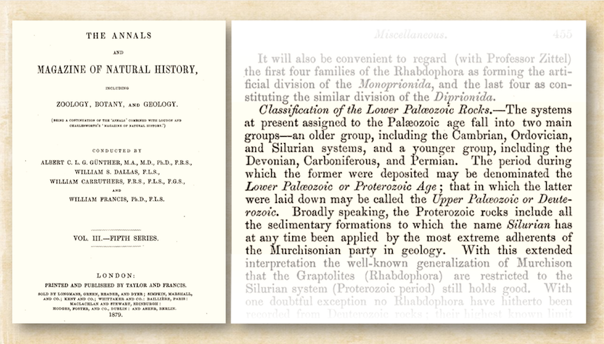
Notice that in Figure 1.6 the Proterozoic Eon precedes the Phanerozoic Eon. This was not always the case. Figure 1.7 shows an excerpt from a periodical published in 1879, in which the Proterozoic is defined as covering the Cambrian through Silurian. The author refers to “the most extreme adherents of the Murchisonian party in geology,” a reference to the contentious assertion by Scottish geologist Roderick Murchison (1792-1871) that the Silurian Period should encompass the Cambrian and Ordovician periods as well.
A Way To Think About Geological Time
A useful mechanism for understanding geological time is to scale it down into one year. The origin of the solar system and Earth at 4.57 Ga would be represented by January 1, and the present year would be represented by the last tiny fraction of a second on New Year’s Eve. At this scale, each day of the year represents 12.5 million years; each hour represents about 500,000 years; each minute represents 8,694 years; and each second represents 145 years. Some significant events in Earth’s history, as expressed on this time scale, are summarized in Table 1.2.
| Table 1.2 Some Important Dates Expressed As If All of Geological Time Were Condensed Into One Year | ||
|---|---|---|
| Event | Approximate Date | Calendar Equivalent |
| Formation of oceans and continents | 4.5 – 4.4 Ga | first week of January |
| Evolution of the first primitive life forms | 3.8 Ga | end of February |
| Formation of Saskatchewan’s oldest rocks | 3.4 Ga | end of March |
| Evolution of the first multi-celled animals | 600 Ma | beginning of November |
| Animals first crawled onto land | 360 Ma | end of November |
| Vancouver Island reached North America and the Rocky Mountains were formed | 90 Ma | December 16 |
| Extinction of the non-avian dinosaurs | 65 Ma | December 18 |
| Beginning of the Pleistocene ice age | 2 Ma | 10:10 p.m., December 31 |
| Oldest radiocarbon date from people living in Canada (British Columbia) | 13.8 ka | 11:58 p.m., December 31 |
| Earliest evidence of human activity in Saskatchewan | 11.5 ka | 48 seconds before midnight, December 31 |
| The last of the glacial ice retreats from Saskatchewan | 6 ka | 41 seconds before midnight, December 31 |
| Hudson’s Bay Company establishes a permanent settlement at Cumberland House in northern Saskatchewan | 243 years ago | 2 seconds before midnight, December 31 |
| Source: Karla Panchuk (2017) CC BY 4.0, modified after Steven Earle (2015) CC BY 4.0 view original | ||
Uniformitarianism
Uniformitarianism is the notion that the geological processes occurring on Earth today are the same ones that occurred in the past. This is an important idea because it means that observations we make today about geological processes can be used to interpret and understand the rock record. While this idea might not seem remarkable today, it was ground breaking and even controversial for its time. Many people who heard about it for the first time thought about the age of the Earth in thousands of years, but uniformitarianism required them to think on timescales almost too vast to comprehend. For some, this implied questioning their most deeply held religious beliefs.
The Scottish geologist James Hutton initially presented the idea in 1785[footnote]Read James Hutton’s abstract at http://bit.ly/1j6tIAN. Note that the typeface prints an “s” like an “f.” [/footnote]. Charles Lyell, also a Scottish geologist, paraphrased this idea as “the present is the key to the past” in his book Principles of Geology.[footnote]The 7th edition of Charles Lyell’s Principles of Geology (1847) can be found at http://bit.ly/1l3T6Zh[/footnote] This is how it is often described today.
To be clear, “the present is the key to the past” can be viewed as an oversimplification. Not all geological processes occurring today occurred at all times in the geological past. For example, some important chemical reactions that happened on Earth’s surface today require abundant oxygen in the atmosphere, and could not have occurred prior to Earth developing an oxygen-rich atmosphere. Conversely, there was a time in Earth’s history when continents as we know them hadn’t yet developed. Some events, such as devastating impacts by objects from space, have never been witnessed on the same scale by humans. We must be cognizant of the fact that conditions were different at different times in Earth’s history, and take that into account when interpreting the rock record.
Despite the different past conditions on Earth as a whole, there still exist environments today where some of these conditions are present. These environments are like little samples of what Earth used to be like. This means we can still use present conditions to inform us about the past, but we have to think carefully about ways that such environments today differ from the ancient environments that no longer exist.
Plate Tectonics
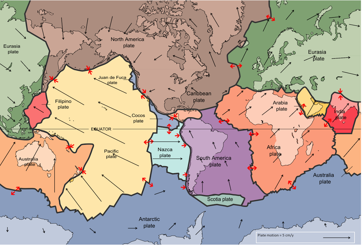
It is only within the last 50 years or so that we have been able to answer questions like, “How did that mountain range get there?” and “Why do earthquakes happen where they do?” The theory of plate tectonics– the idea that Earth’s surface is broken into large moving fragments, called plates– profoundly changed our perspective on how the Earth works. Figure 1.8 shows Earth’s 15 largest tectonic plates, along with arrows indicating the plates’ direction of motion, and how fast they go. (Longer arrows mean faster motion.) There are many more plates on Earth that are too small to show conveniently in Figure 1.8. A more detailed map of Earth’s tectonic plates can be found at here.
Prior to plate tectonics, we made observations but could only guess at mechanisms. It was like watching the hands on a clock and trying to guess what moves them. After plate tectonics it was like being able to open the clock and not only watch the gears turn, but realize for the first time that there are such things as gears. Plate tectonics not only explains why things have happened, but also allows us to predict what might happen in the future.
Plate tectonics is covered in more detail later, however the key point is that Earth’s outer layer consists of rigid plates that are constantly interacting with each other as they move around the Earth. The boundaries of plates move away from each other in some places, collide in others, and sometimes just slide past each other (illustrated by the red arrows in Figure 1.8). The plates can move because they are floating on a layer of weak rock that deforms as the plates travel, much the same way the filling in a peanut butter and jelly sandwich allows you to slide the top layer of bread across the bottom layer.
Whether the plates move away from each other, collide, or just slide past each other determines things like the locations of mountain belts and volcanoes, where earthquakes happen, and the shapes and sizes of oceans and continents.
References
Cottrell, M. (2006) History of Saskatchewan. Retrieved 26 August 2017. Visit the website
Chapter 1 Summary
The topics covered in this chapter can be summarized as follows:
1.1 What is Geology?
Geology is the study of Earth. It is an integrated science that involves the application of many of the other sciences. Geologists must take into account the fact that the geological features we see today may have formed thousands, millions, or even billions of years ago, and over very long time spans.
1.2 Why Study Earth?
Geologists study Earth out of curiosity and for other, more practical reasons, including understanding the evolution of life on Earth; searching for resources; understanding risks from geological events such as earthquakes, volcanoes, and slope failures; and documenting past environmental and climate changes so that we can understand how human activities are affecting Earth.
1.3 What Do Geologists Do?
Geologists work in the resource industry, and in efforts to protect the environment. Geologists work to minimize the risks from geological hazards (e.g., earthquakes), and to help the public understand those risks. Geologists investigate Earth materials in the field, in and in the lab.
1.4 We Study Earth Using the Scientific Method
Scientific inquiry requires a careful process of making a hypothesis and then testing it. If a hypothesis doesn’t pass the test, it’s time for a new one. A theory is a hypothesis that has been tested repeatedly and never failed a test. A law is a description of a natural process.
1.5 Three Big Ideas: Geological Time, Uniformitarianism, and Plate Tectonics
Geological time: Earth is approximately 4,570,000,000 years old; that is, 4.57 billion years or 4.57 Ga or 4,570 Ma. It’s such a huge amount of time that even extremely slow geological processes can have an enormous impact.
Uniformitarianism: Processes that occur today also occurred in the geologic past. We can use our observations of the present to understand the processes that shaped the Earth throughout its history.
Plate tectonics: Earth’s surface is broken into plates that move and interact with each other. The interactions between these plates are key for understanding the mechanisms behind geologic processes.
Review Questions
- How does the element of time make geology different from the other sciences, such as chemistry and physics?
- List three ways in which geologists can contribute to society.
- The following dates are written with the abbreviations Ga, Ma, and ka. Express the dates in years. (For example, 2.3 Ma = 2,300,000 years)
- 2.75 ka
- 0.93 Ga
- 4.2 Ma
- 0.2 ka.
- Dinosaurs first appear in the geological record in rocks from about 215 Ma and then most became extinct at 65 Ma. What percentage of geological time does this represent?
- If sediments typically accumulate at a rate of 1 mm/year, what thickness of sediment could accumulate over a period of 30 million years?
- Does uniformitarianism mean that conditions on Earth are uniform, and never change?
- Summarize the main idea behind plate tectonics.
Answers to Chapter 1 Review Questions
- Geology requires that we consider vast amounts of time, and think about the effects that accumulate over thousands, millions, or even billions of years.
- There are many ways that geologists contribute. Geologists provide information to reduce the risk of harm from hazards such as earthquakes, volcanoes, and slope failures; they play a critical role in the discovery of important resources; they contribute to our understanding of life and its evolution through paleontological studies; and they play a leading role in the investigation of climate change, past and present and its implications.
- Ages in years
- 2.75 ka = 2,750 years
- 0.93 Ga = 930,000,000 years
- 14.2 Ma = 14,200,000 years
- 0.2 ka = 200 years.
- 215 – 65 = 150 Ma. Since the age of the Earth is 4570 Ma, this represents 150/4,570 = 0.033 or 3.3% of geological time.
- At 1 mm/y 30,000,000 mm of sediment would accumulate over that 30 million years. This is equivalent to 30,000 m or 30 km. Few sequences of sedimentary rock are even close to that thickness because most sediments accumulate at much lower rates, more like 0.1 mm/y. Also, over time the sediments are compressed.
- No. Uniformitarianism means that we can use the processes we observe today to help us understand what happened in the past.
- Plate tectonics is the idea that Earth’s outer layer is broken into rigid plates. The plates move around and interact with each other along their margins.
8.1 Mechanical Weathering
Intrusive igneous rocks form at depths of 100s of metres to 10s of kilometres. Sediments are turned into sedimentary rocks only when they are buried by other sediments to depths in excess of several 100s of metres. Most metamorphic rocks are formed at depths of kilometres to 10s of kilometres. Weathering cannot occur until these rocks are revealed at Earth’s surface by uplift and the erosion of overlying material. Once the rock is exposed at the surface as an outcrop, weathering can begin.
The agents of mechanical weathering can be broadly classified into two groups: Those things which cause the outer layers of a rock to expand, and those things which act like wedges to force the rock apart.
Mechanical Weathering By Expansion
Rock on Earth’s surface responds to deformation by breaking. When the outer layer of a rock expands but the inner part does not, the result is a crack to accommodate the difference. The slabs of rock in Figure 8.2 were formed in this way, breaking off from the surface beneath. When layers break off a rock in this way, it’s referred to as exfoliation.
Granitic rock tends to exfoliate parallel to the exposed surface because it is typically homogeneous, meaning that it doesn’t contain predetermined planes of weakness. In contrast, sedimentary and metamorphic rocks tend to exfoliate along predetermined planes.
![Exfoliation of a granite dome in the Enchanted Rock State Natural Area, Texas, USA. [Photo: Wing-Chi Poon CC-BY-SA]](https://openpress.usask.ca/app/uploads/sites/29/2017/05/GeologicalExfoliationOfGraniteRock.jpg "Chapter 1. Introduction to Geology")
Confining pressure refers to the pressure on a rock resulting from other rocks being on top of it and around it. When a mass of rock is exposed by weathering and removal of the overlying rock, there is a decrease in the confining pressure and the rock expands. The cracking that results is sometimes referred to as pressure-release cracking.
Figure 8.3 is an example of exfoliation due to a decrease in confining pressure. The exfoliation is easiest to see in the middle of the photograph.
![Exfoliation fractures in granitic rock exposed on the west side of the Coquihalla Highway north of Hope, B.C. [SE]](https://openpress.usask.ca/app/uploads/sites/29/2017/05/image005.jpg "Chapter 1. Introduction to Geology")
Mechanical Weathering By Wedging
In wedging a pre-existing crack in a rock is forced open and made larger.
Frost wedging happens when water seeps into cracks, then expands upon freezing. The expansion enlarges the cracks (Figure 8.4). The effectiveness of frost wedging depends on how often freezing and thawing occur. Frost wedging won’t be as important in warm areas where freezing is infrequent, in very cold areas where thawing is infrequent, or in very dry areas, where there is little water to seep into cracks.
![The process of frost wedging on a steep slope. Water gets into fractures and then freezes, expanding the fracture a little. When the water thaws it seeps a little farther into the expanded crack. The process is repeated many times, and eventually a piece of rock will be wedged away. [SE]](https://openpress.usask.ca/app/uploads/sites/29/2017/05/image009.png "Chapter 1. Introduction to Geology")
![An area with very effective frost-wedging near Keremeos, B.C. The fragments that have been wedged away from the cliffs above have accumulated in a talus deposit at the base of the slope. The rocks in this area have quite varied colours, and those are reflected in the colours of the talus. [SE]](https://openpress.usask.ca/app/uploads/sites/29/2017/05/image011.jpg "Chapter 1. Introduction to Geology")
Salt crystals grow within cracks and pores in the rock, and the growth of these crystals can push grains apart, causing the rock to weaken and break. There are many examples of this on the rocky shorelines of Vancouver Island and the Gulf Islands, where sandstone outcrops are common and salty seawater is readily available (Figure 8.6). The honeycomb structure in Figure 8.5 is related to the original roughness of the surface. Low spots collect salt water, causing the effect to be accentuated around existing holes.
![Honeycomb weathering of sandstone on Gabriola Island, B.C. The holes are caused by crystallization of salt within rock pores, and the seemingly regular pattern is related to the original roughness of the surface. It’s a positive-feedback process because the holes collect salt water at high tide, and so the effect is accentuated around existing holes. This type of weathering is most pronounced on south-facing sunny exposures. [SE]](https://openpress.usask.ca/app/uploads/sites/29/2017/05/image013.jpg "Chapter 1. Introduction to Geology")
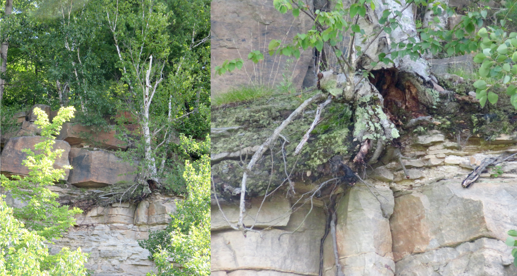
Figure 8.6 Honeycomb weathering of sandstone on Gabriola Island BC. The holes are caused by crystallization of salt within rock pores. [Steven Earle CC-BY 4.0]The effects of plants and animals are significant in mechanical weathering. Roots can force their way into even the tiniest cracks. They exert tremendous pressure on the rocks as they grow, widening the cracks and breaking the rock. This is called root wedging (Figure 8.7).
Although animals do not normally burrow through solid rock, they can excavate and remove huge volumes of soil, and thus expose the rock to weathering by other mechanisms.
Gravity is not the only way weathering products are removed. Other agents of erosion which remove the products of weathering include water in streams, ice in glaciers, and waves on coasts.
Exercise 8.1 Mechanical Weathering
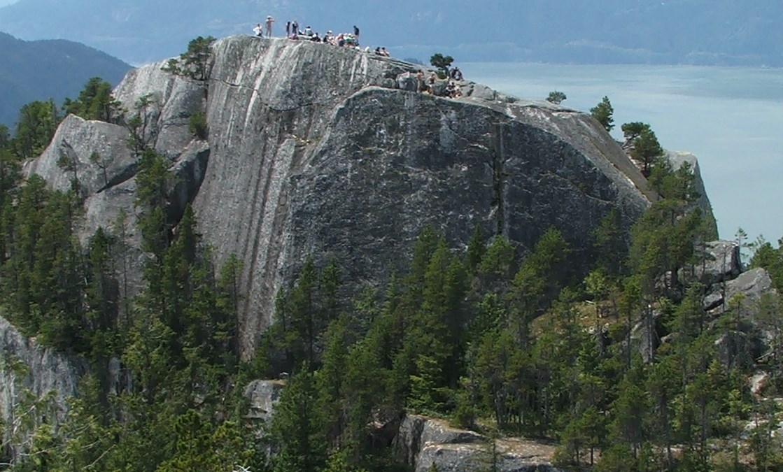
This photo shows granitic rock at the top of Stawamus Chief near Squamish, B.C. Identify the mechanical weathering processes that you can see taking place, or that you think probably take place at this location.
8.2 Chemical Weathering
Chemical weathering results from chemical changes to minerals that become unstable when they are exposed to surface conditions. The kinds of changes that take place are specific to the mineral and the environmental conditions. Some minerals, like quartz, are virtually unaffected by chemical weathering. Others, like feldspar, are easily altered.
Types of Chemical Weathering Reactions
Dissolution
Dissolution reactions produce ions, but no minerals. A household example would be dissolving a teaspoon of table salt (the mineral halite) in a glass of water. Some minerals will dissolve in water alone. In addition to halite these minerals include gypsum and anhydrite.
Other minerals, such as calcite, will dissolve in acidic water. Acidic water is easier to come by than you might think, because carbon dioxide (CO2) reacts with water in the atmosphere, on land, and in the oceans to produce carbonic acid as follows (Figure 8.8):
![An example of weathering by dissolution. Top: Carbon dioxide reacts with water to make acid. Bottom: Acid reacts with calcite and produces ions. [Karla Panchuk CC-BY 4.0 modified after http://what-when-how.com/paramedic-care/ventilation-clinical-essentials-paramedic-care-part-2/]](https://openpress.usask.ca/app/uploads/sites/29/2017/05/dissolution_rxn1.png "Chapter 1. Introduction to Geology")
Calcite is a major component of the sedimentary rock called limestone (typically more than 95%). In the presence of acidic groundwater, limestone can dissolve underground. Over time the dissolution can remove enough of the calcite to form caves.
If dissolution of limestone or other materials removes enough rock to undermine support near the surface, the surface may collapse, creating a sinkhole such as the one in Figure 8.10, downstream of the Mosul Dam in Iraq.

Although the sinkhole in Figure 8.9 might appear minor, it reflects a serious problem. The dam itself is constructed on limestone supported by beds of gypsum and anhydrite. Gypsum and anhydrite are soluble in water, and the gypsum and anhydrite beneath the dam are rapidly dissolving away. This was the case prior to construction of the dam. However, once the dam was filled the increased water pressure began to force water through the formations much faster, accelerating dissolution. At present there is a grave risk of catastrophic failure, placing nearly 1.5 million people at risk.
Hydrolysis
The term hydrolysis combines the prefix hydro, referring to water, with lysis, which is derived from a Greek word meaning to loosen or dissolve. Thus, you can think of hydrolysis as a chemical reaction where water loosens the chemical bonds within a mineral. This might sound the same as dissolution but the difference is that hydrolysis produces a different mineral in addition to ions. An example of hydrolysis is when water reacts with potassium feldspar to produce clay minerals and ions:
Hydrolysis Reaction of Potassium Feldspar
2KAlSi3O8 + 3H2O → Al2Si2O5(OH)4 + 4SiO2 + 2K+ + 2OH–
Potassium feldspar is broken down by water to produce kaolinite (a clay mineral), quartz, and ions.
The hydrolysis of feldspar to clay is illustrated in Figure 8.10, which shows two surfaces of the same granite sample. On the left is a recently broken unweathered surface, where feldspar is visible as white crystals. On the right is a weathered surface where the feldspar has been altered to the chalky-looking clay mineral kaolinite.
![Unweathered (left) and weathered (right) surfaces of the same piece of granite. On the unweathered surfaces the feldspars are still fresh and glassy-looking. On the weathered surface the feldspar has been altered to the chalky-looking clay mineral kaolinite. [Steven Earle CC-BY 4.0]](https://openpress.usask.ca/app/uploads/sites/29/2017/05/granitic-rock.png "Chapter 1. Introduction to Geology")
Hydration
Hydration reactions involve water being added to the chemical structure of a mineral. An example of a hydration reaction is when anhydrite is transformed into gypsum. A consequence of hydration is that the resulting mineral has a greater volume than the original mineral. In the case of the Mosul Dam, hydration of anhydrite has important consequences. The increase in volume put force on the overlying limestone layer, breaking it into pieces. While unbroken limestone is a strong enough material upon which to build a foundation, the broken limestone is too weak to provide a safe foundation.
Oxidation
Oxidation happens when free oxygen (i.e., oxygen not bound up in molecules with other elements) is involved in chemical reactions. Oxidation reactions provide valuable insight into Earth’s early surface conditions because there is a clear transition in the rock record from rocks containing no minerals that are products of oxidation reactions, to rocks containing abundant minerals produced by oxidation. This reflects a transition from an oxygen-free atmosphere to an oxygenated one.
In iron-rich minerals such as olivine, the oxidation reaction begins with taking iron out of the mineral and putting it into solution as an ion. Once it’s an ion, oxygen reacts with it. The steps in the reaction for olivine are shown below.
Oxidation Reaction of Olivine to Hematite
Fe2SiO4 + 4H2CO3 → 2Fe2+ + 4HCO3– + H4SiO4
Olivine reacts with carbonic acid, leaving dissolved iron, bicarbonate, and silicic acid.
2Fe2+ + ½ O2 + 2H2O + 4HCO3– → Fe2O3 + 4H2CO3
Iron and oxygen dissolved in water react in the presence of bicarbonate to produce hematite and carbonic acid.
The oxidation reaction would be similar for other iron-containing silicate minerals such as pyroxene, amphibole, and biotite. Iron in sulphide minerals (e.g., pyrite, FeS2) can also be oxidized in this way.
The mineral hematite is not the only possible end result of oxidation. There is a wide range of iron oxide minerals that can form in this way. For example, Figure 8.11 shows granite in which some of the biotite and amphibole have been altered to form the iron oxide minerals in limonite [footnote]Limonite isn’t technically a mineral. It is a way to refer to iron oxide minerals which occur together in a mass, without being specific about what those minerals are.[/footnote] (the yellowish colour).
![Granite containing biotite and amphibole which have been altered near to the rock’s surface to limonite (yellow), which is a mixture of iron oxide minerals. [Steven Earle CC-BY 4.0]](https://openpress.usask.ca/app/uploads/sites/29/2017/05/image023.jpg "Chapter 1. Introduction to Geology")
Oxidation Reactions and Acid Rock Drainage
Oxidation reactions can pose an environmental problem in areas where rocks have elevated levels of sulphide minerals such as pyrite, because a by-product of the reaction is sulphuric acid.
The runoff from areas where this process is taking place is known as acid rock drainage (ARD), and even a rock with 1% or 2% pyrite can produce significant ARD. Some of the worst examples of ARD are at metal mine sites, especially where pyrite-bearing rock and waste material have been mined from deep underground and then piled up and left exposed to water and oxygen. In these cases the problem is referred to as acid mine drainage. One example is the Mt. Washington Mine near Courtenay on Vancouver Island (Figure 8.12), but there are many similar sites across Canada and around the world.
![Acid mine drainage. Left: Mine waste where exposed rocks undergo oxidation reactions and generate acid at the Washington Mine, B.C. Right: an example of acid drainage downstream from the mine site. [Steven Earle CC-BY 4.0]](https://openpress.usask.ca/app/uploads/sites/29/2017/05/Mt.-Washington-Mine.png "Chapter 1. Introduction to Geology")
Exercise 8.2 Chemical Weathering
For each of the reactions in the table below, indicate which of the chemical weathering processes- dissolution, hydrolysis, hydration, or oxidation- is primarily responsible.
| Chemical Change | Process? |
| Pyrite to hematite | |
| Calcite to calcium and bicarbonate ions | |
| Feldspar to clay | |
| Olivine to serpentine | |
| Anhydrite to gypsum | |
| Pyroxene to iron oxide |
Controls on Weathering Processes and Rates
Weathering does not happen at the same rate in all environments. The same types of weathering do not happen in all environments. There are a variety of factors that determine what kinds of weathering will occur, and how fast the processes will proceed.
Climate
Water and temperature are key factors controlling both weathering rates and the types of weathering that happen. For example:
- Water is required for chemical weathering reactions to occur.
- Water must be present for ice wedging to happen.
- Higher temperatures speed up chemical reactions.
- Climate will determine whether water is present mostly in liquid form, solid form (ice), or as both.
- Climate will determine what plant life is available to force rocks apart with their roots, and to contribute organic acids to soils to aid in chemical weathering.
This means, for example, that chemical weathering will be faster in a tropical rainforest than in the Antarctic, a cold desert. It means physical weathering will be the predominant form of weathering in the Antarctic.
Oxygen and Carbon Dioxide
The presence and abundance of oxygen and carbon dioxide affect chemical weathering rates. Surface environments on Earth almost all have some oxygen, permitting oxidation reactions to take place. Exceptions are in settings such as deep lakes or swamps where oxygen cannot easily mix into the water, or biological processes use it up rapidly.
Carbon dioxide, which acidifies water and contributes to chemical weathering, is everywhere, but more concentrated in some settings than others. For example, soils can have very high concentrations of carbon dioxide, whereas carbon dioxide concentrations will be lower on surfaces free of soils and exposed to the atmosphere.
Minerals
The minerals making up a rock will determine what kinds of chemical weathering reactions are possible. Under the same conditions, dissolution reactions happening to calcite making up limestone will occur more rapidly than hydrolysis reactions happening to feldspar in granite.
Some minerals are very resilient to chemical weathering in general compared to others. For example, quartz is very resilient to chemical weathering whereas calcite is not. Under the same conditions, a rock with grains cemented together with calcite will weather faster than a rock with grains cemented together with quartz.
When rocks in an outcrop weather at different rates, the result is differential weathering. In Figure 8.13 some of the beds are recessed further into the outcrop than others. The recessed beds are weathering faster than the surrounding beds.
![Differential weathering in an outcrop along the Blaeberry River near Golden BC. The recessed beds within the outcrop are weathering faster than the surrounding beds. [Karla Panchuk CC-BY 4.0]](https://openpress.usask.ca/app/uploads/sites/29/2017/05/differential_weathering.jpg "Chapter 1. Introduction to Geology")
Weathering Makes Weathering Go Faster
Weathering accelerates weathering. Physical weathering breaks rocks into smaller pieces or forms cracks. Newly exposed surfaces can be acted upon by chemical weathering, and physical weathering processes such as wedging can expand cracks further. Chemical weathering weakens rock making it more susceptible to physical weathering processes.
8.3 Weathering and Erosion Produce Sediments
The visible products of weathering and erosion are the unconsolidated materials that we find around us on slopes, beneath glaciers, in stream valleys, on beaches, and in deserts. The loose collection of material is referred to as sediment, and the individual pieces that make it up are clasts. Clasts can be sand-sized and smaller (in which case they might be referred to as particles or grains), or larger than a house.
Some examples of sediments and their clasts are shown in Figure 8.14. They range widely in size and shape depending on the processes involved. If and when deposits like these are turned into sedimentary rocks, the textures of those rocks will vary significantly. When we describe sedimentary rocks that formed millions of years in the past, we can use those properties to make inferences about the conditions that existed during their formation. The properties we look at are composition, grain-size, sorting, rounding, and sphericity.
![Products of weathering and erosion formed under different conditions. [Steven Earle CC-BY 4.0]](https://openpress.usask.ca/app/uploads/sites/29/2017/05/weathering-and-erosion.png "Chapter 1. Introduction to Geology")
Composition
Composition refers to the mineral or minerals making up the clast. Small clasts may be single mineral grains, but larger ones can have several different mineral grains, or even several different pieces of rock within them. The composition can tell us something about what rock the sediments came from and, as you’ll learn later, it can also tell us something about the geological setting in which that rock formed.
Not all minerals have the same hardness and resistance to weathering, so some minerals tend to become more abundant than others within sediments as weathering and erosion proceed.
Quartz is one example of a mineral that is more abundant. It is highly resistant to weathering by weak acids or reaction with oxygen. This makes it unique among the minerals that are common in igneous rocks. Quartz is also very hard, so it is resistant to mechanical weathering.
In contrast, ferromagnesian minerals and feldspar are not as resistant to weathering. As weathering proceeds, they are likely to be broken into small pieces and converted into clay minerals and dissolved ions (e.g., Ca2+, Na+, K+, Fe2+, Mg2+, and H4SiO4). Ultimately this means that quartz, clay minerals, and dissolved ions are the most common products of weathering.
Grain Size
Whether a grain is large or small tells us something about its journey to where we’ve found it. To begin with, mechanical weathering can break off large pieces of rock. Large pieces of rock carried along by streams will bump into each other, causing smaller pieces to break off. Over time the grains get smaller and smaller still. If the grains are all very small, we can conclude that they are a long way from home.
Geologists have a specific set of definitions to describe the size of grains. Table 8.1 below is a simplified version of the scale that is used.[footnote]View an example of the Wentworth scale for grain classification at http://bit.ly/UWscale.[/footnote]
![A simplified definition of clast sizes. Silt and clay are considered fine-grained particles, sand is medium-grained, and particles larger than sand are considered coarse-grained. [Karla Panchuk CC-BY 4.0]](https://openpress.usask.ca/app/uploads/sites/29/2017/05/Grain-size-chart-300x172.png "Chapter 1. Introduction to Geology")
One other thing to notice about this scale is that the finest-grained particle is referred to as clay. While a clay-sized particle could be composed of clay minerals (and often they are), it doesn’t have to be. Any particle of that size would be referred to as clay.
Grain Size and Transportation
The grain size of sediments is not just for purposes of description. It’s also a valuable clue to the processes that have acted on those sediments, because the size of the clast determines how much energy is required to move it.
Whether or not a medium such as water or air has the ability to move a clast of a particular size and keep it moving depends on the velocity of the flow. The faster the medium flows, the larger the clasts that can be moved. Figure 8.15 shows a streambed that now contains only a trickle of water- barely enough to move particles of silt and cool puppy feet. But the velocity of water in the stream changes from season to season, as does the volume of water. All of the clasts in the streambed have been transported there by water.
![Ruby looks upstream in a channel near Golden BC. For much of the year the only water in the stream is the trickle in which Ruby stands, but in the spring the water flows rapidly enough to carry boulders. [KP]](https://openpress.usask.ca/app/uploads/sites/29/2017/05/IMG_4497-1024x871.jpg "Chapter 1. Introduction to Geology")
Sorting
Weathering can break off large fragments of rock. It can also make smaller fragments. The extent to which the grains in sediment differ in size is described by sorting.
If the grains in a sample of sediment are the same size or very nearly so, the sediments are said to be well sorted. If the grains are vary substantially in size, the sediments are poorly sorted. If they are somewhere in between, then they are moderately sorted. Examples of these are shown in the upper part of Figure 8.16[footnote]Figure 5 of Reagan, M.K., Pearce, J.A., Petronotis, K., and the Expedition 352 Scientists, 2015, Proceedings of the International Ocean Discovery Program, Volume 352, publications.iodp.org, doi:10.14379/iodp.proc.352.102.2015[/footnote]. Because grains become progressively smaller as they are transported, sorting improves the further the sediments are from their source.
![Top: Sorting of grains, ranging from well-sorted where the grains are similar in size, to poorly sorted, where the grains vary greatly in size. Bottom: Rounding refers to how smooth or rough the edges of a clast are. Clasts with sharp edges and corners are angular. Clasts with smooth surfaces are rounded. Clasts which fall in between are sub-angular or sub-rounded. [IODP CC-BY-SA. See footnotes for full citation.]](https://openpress.usask.ca/app/uploads/sites/29/2017/05/IODP-sorting-and-rounding.png "Chapter 1. Introduction to Geology")
Rounding
Rounding refers to whether clasts have sharp edges and corners or not. If the grains are rough, with lots of edges and corners, then they are referred to as angular. Grains with smooth surfaces are rounded. Grains in between can be sub-angular or sub-rounded. Examples of these are shown in the row of boxes at the bottom of Figure 8.16.
Sphericity
Sphericity describes whether a grain is elongate or not. Grains that are longer than they are wide (like an ellipse) have low sphericity, whereas grains that have the same diameter no matter where you measure it (like a sphere) are high sphericity. In the bottom row of boxes in Figure 8.16 the grains at the top of each box would be considered high sphericity, and the grains at the bottom would be low sphericity. Notice that a grain can be angular but still have high sphericity. It can be rounded, but still have low sphericity.
Exercise 8.3 Looking at Sand
Three samples of sand are shown below, along with information about what they contain and where they are from. Describe each sample in terms of grain size, sorting, rounding, and sphericity, and then suggest a mechanical weathering mechanism that might have produced them.
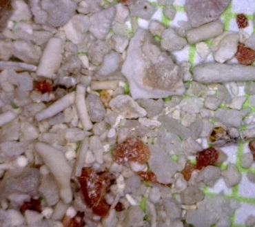
![Quartz and rock fragments from a glacial stream deposit near Osoyoos, B.C. The grains are between 0.25 and 0.5 mm across. [SE]](https://openpress.usask.ca/app/uploads/sites/29/2017/05/image041.jpg "Chapter 1. Introduction to Geology")
![Grains of olivine (green) and volcanic glass (black) from a beach on the big island of Hawaii. The grains are approximately 1 mm across. [SE]](https://openpress.usask.ca/app/uploads/sites/29/2017/05/image043.jpg "Chapter 1. Introduction to Geology")
8.4 Weathering and Soil Formation
Weathering is a key part of the process of soil formation, and soil is critical to our existence on Earth. In other words, we owe our existence to weathering, and we need to take care of our soil!
Many people refer to any loose material on Earth’s surface as soil, but to geologists (and geology students) soil is the material that includes organic matter, lies within the top few tens of centimetres of the surface, and is important for sustaining plant growth.
Soil is a complex mixture of minerals (~45%), organic matter (~5%), and empty space (~50%, filled to varying degrees with air and water). The mineral content of soil varies, but is dominated by clay minerals and quartz, along with minor amounts of feldspar and small fragments of rock.
The types of weathering that take place within a region have a major influence on soil composition and texture. For example, in a warm climate where chemical weathering dominates, soils tend to be richer in clay. Soil scientists describe soil texture in terms of the relative proportions of sand, silt, and clay, as shown in Figure 8.17. The sand and silt components in this diagram are dominated by quartz, with lesser amounts of feldspar and rock fragments, while the clay component is dominated by the clay minerals.
![Soil texture classification determined by grain size. [Mike Norton after USDA, CC-BY-SA http://bit.ly/USDAsoil]](https://openpress.usask.ca/app/uploads/sites/29/2017/05/image045.png "Chapter 1. Introduction to Geology")
Factors Affecting How Soil Forms
Soil forms through accumulation and decay of organic matter and through the mechanical and chemical weathering processes described previously. The factors that affect the nature of soil and the rate of its formation include:
- Climate, especially average temperature and precipitation amounts, and the consequent types of vegetation
- Parent material (what was weathered to get the soil)
- The slope of the surface where soil is accumulating
- How long soil has been forming
Climate
Both the mechanical breakup of rocks and the chemical weathering of minerals contribute to soil formation. It is also helped by the downward percolation of water. Soil forms most readily under temperate to tropical conditions (not cold) and where precipitation amounts are moderate (not dry, but not too wet). Temperature matters because chemical weathering reactions and reactions facilitated by organisms proceed fastest under warm conditions, and plant growth is enhanced in warm climates. Where the climate is cooler, chemical weathering is slowed when water is frozen, and not available for chemical reactions.
Although water is needed for chemical weathering to take place, too much water can lead to soils that are less than ideal. In rain forests, for example, the large amount of water leaches away important nutrients and leaves behind acidic soils. In humid and poorly drained regions, swampy conditions may prevail, producing soil that is dominated by organic matter, and with too little of inorganic nutrients.
Too little water (e.g., in deserts and semi-deserts) limits the rate of downward chemical transport, and it also means salts and carbonates in water moving upward can be left behind and build up. These soils also lack organic matter (Figure 8.18).
![Poorly developed soil on wind-blown silt (loess) in an arid part of northeastern Washington State [Steven Earle CC-BY 4.0]](https://openpress.usask.ca/app/uploads/sites/29/2017/05/image047.jpg "Chapter 1. Introduction to Geology")
Parent Material
Parent material for soils can be all different types of bedrock, and any type of unconsolidated sediments, such as glacial deposits and stream deposits. Soils are described as residual soils if they develop on bedrock, and transported soils if they develop on transported material such as glacial sediments. This doesn’t mean that the soils themselves have been transported, but that the soil developed on unconsolidated material rather than bedrock.
Quartz-rich parent material, such as granite, sandstone, or loose sand, leads to the development of sandy soils. Quartz-poor material, such as shale or basalt, generates soils with little sand.
Parent materials provide important nutrients to residual soils. For example, a minor constituent of granitic rocks is the calcium-phosphate mineral apatite, which is a source of the important soil nutrient phosphorus. Basaltic parent material tends to generate very fertile soils because, in addition to phosphorus, it provides significant amounts of iron, magnesium, and calcium. This is a result of minerals such as olivine ((Mg,Fe)2SiO4) and plagioclase feldspar (CaAl2Si2O8) in the basalt.
Some unconsolidated materials, such as river-flood deposits, make for especially good soils because they tend to be rich in clay minerals. Clay minerals have large surface areas with negative charges that are attractive to positively charged elements like calcium, magnesium, iron, and potassium — important nutrients for plant growth.
Slope
Soil can only develop where surface materials remain in place and are not frequently moved away by mass wasting (sediments taken away by gravity). Soils cannot develop where the rate of soil formation is less than the rate of erosion, so steep slopes tend to have little or no soil.
Time
Even under ideal conditions, soil takes thousands of years to develop. Virtually all of southern Canada was covered with glaciers up until 14,000 years ago, and most of the central and northern parts of BC, the prairies, Ontario, and Quebec were still glaciated at 12,000 years ago. Glaciers remained in the central and northern parts of Canada until around 10,000 years ago, so conditions were still not ideal for soil development even in the southern regions. This means that soils in Canada, particularly in central and northern Canada, are relatively young and not well developed.
The same applies to soils that are forming on newly created surfaces, such as recent deltas or sand bars, or in areas of mass wasting.
Because soil takes so long to form, human activities that damage soils will have consequences for the long term, and for generations to come.
Soil Horizons
The process of soil formation generally involves the downward movement of clay, water, and dissolved ions. A common result of is the development of chemically and texturally distinct layers known as soil horizons. The horizons that typically develop, as illustrated in Figure 8.16, are:
O horizon— A layer of organic matter
A horizon— Partially decayed organic matter mixed with mineral material
E horizon— the eluviated (leached) layer from which some of the clay and iron have been removed to create a pale layer that may be sandier than the other layers
B horizon— Where clay, iron, and other elements from the overlying soil accumulate
C horizon— Weathering of the underlying bedrock or sediments is not yet complete
![Soil horizons in a podsol from a site in northeastern Scotland. O: organic matter A: organic matter and mineral material E: leached layer B: accumulation of clay, iron etc. C: incomplete weathering of parent material [SE after http://bit.ly/1PscHuy]](https://openpress.usask.ca/app/uploads/sites/29/2017/05/image049.png "Chapter 1. Introduction to Geology")
How Soil Is Lost
Like all geological materials, soil is subject to erosion. Under natural conditions on gentle slopes, the rate of soil formation either balances or exceeds the rate of erosion. However, human practices related to forestry and agriculture have significantly upset this balance.
Soils are held in place by vegetation. When vegetation is removed, either through cutting trees or routinely harvesting crops and tilling the soil, that protection is either temporarily or permanently lost. When soil is not protected, wind and water can erode it away.
Water erosion is accentuated on sloped surfaces because fast-flowing water has greater eroding power than still water (Figure 8.20). Raindrops can disaggregate exposed soil particles, putting the finer material (e.g., clays) into suspension in the water. Sheetwash, unchannelled flow across a surface, carries suspended material away, and channels erode right through the soil layer, removing both fine and coarse material.
![Soil erosion by rain and channelled runoff on a field in Alberta. [from Alberta Agriculture and Rural Development, http://bit.ly/1UU0cM0, used with permission]](https://openpress.usask.ca/app/uploads/sites/29/2017/05/image051.jpg "Chapter 1. Introduction to Geology")
Tillage is also a factor in soil erosion, especially on slopes, because each time the soil is lifted by a cultivator, it is moved a few centimetres down the slope.
![Soil erosion by wind in Alberta. [from Alberta Agriculture and Rural Development, http://bit.ly/1UU0cM0, used with permission]](https://openpress.usask.ca/app/uploads/sites/29/2017/05/image053.jpg "Chapter 1. Introduction to Geology")
8.5 The Soils of Canada
Up until the 1950s, the classification of soils in Canada was based on the system used in the United States. However, it was long recognized that the U.S .system did not apply well to many parts of Canada because of climate and environmental differences. The Canadian System of Soil Classification was first outlined in 1955 and has been refined and modified numerous times since then.
There are 10 orders of soil recognized in Canada. Each one is divided into groups, and then families, and then series, but we will only look at the orders, some of which are summarized in Table 8.2. The distribution of these types of soils (and a few others) in Canada is shown in Figure 8.22.
| Order | Brief Description | Environment |
| Forest soils | ||
| Podzol | Well-developed A and B horizons | Coniferous forests throughout Canada |
| Luvisol | Clay rich B horizon | Northern prairies and central B.C., mostly on sedimentary rocks |
| Brunisol | Poorly developed or immature soil, that does not have the well-defined horizons of podsol or luvisol | Boreal-forest soils in the discontinuous permafrost areas of central and western Canada, and also in southern B.C. |
| Grassland soils | ||
| Chernozem | High levels of organic matter and an A horizon at least 10 cm thick | Southern prairies (and parts of B.C.’s southern interior), in areas that experience water deficits during the summer |
| Solonetzic | A clay-rich B horizon, commonly with a salt-bearing C horizon | Southern prairies, in areas that experience water deficits during the summer |
| Other important soils | ||
| Organic | Dominated by organic matter; mineral horizons are typically absent | Wetland areas, especially along the western edge of Hudson Bay, and in the area between the prairies and the boreal forest |
| Cryosol | Poorly developed soil, mostly C horizon | Permafrost areas of northern Canada |
Table 8.2 The nature, origins and distributions of the more important soil orders in Canada
There is an excellent website on Canadian soils, with videos describing the origins and characteristics of the soils, at: http://soilweb.landfood.ubc.ca/classification/.
![The soil order map of Canada. [from The Department of Soil Science, University of Saskatchewan, http://www.soilsofcanada.ca/ used with permission]](https://openpress.usask.ca/app/uploads/sites/29/2017/05/image055.jpg "Chapter 1. Introduction to Geology")
In the grasslands of the dry southern parts of the prairie provinces and in some of the drier parts of southern B.C., dark brown organic-rich chernozem soils are dominant. In some parts of these areas, weak calcification takes place with leaching of calcium from the upper layers and accumulation of calcium in the B layer. Development of caliche layers is rare in Canada.
Organic soils form in areas with poor drainage (i.e., swamps) and a rich supply of organic matter. These soils have very little mineral matter.
In the permafrost regions of the north, where glacial retreat was most recent, the time available for soil formation has been short and the rate of soil formation is very slow. The soils are called cryosols (cryo means “ice cold”). Permafrost areas are also characterized by the churning of the soil by freeze-thaw processes, and as a result, development of soil horizons is very limited.
Exercise 8.4 Soils of Canada
Examine Figure 8.22 showing the distribution of soils in Canada. In the following table briefly describe the distributions of the five soils types listed. For each one, explain its distribution based on what you know about the conditions under which the soil forms and the variations in climate and vegetation related to it.
| Soil type | Describe the Distribution | Explain the Reason for This Distribution |
| Chernozem | ||
| Luvisol | ||
| Podzol | ||
| Brunisol | ||
| Organic |
8.6 Weathering and Climate Change
Carbon cycling on Earth can be thought of in two parts that operate on very different timescales. One part is biological, wherein living organisms — mostly plants — consume carbon dioxide from the atmosphere to make their tissues. After they die, that carbon is released back into the atmosphere when they decay over a period of years or decades. A small proportion of this biological-cycle carbon becomes buried in sedimentary rocks: during the slow formation of coal, as tiny fragments and molecules in organic-rich shale, and as the shells and other parts of marine organisms in limestone. This then becomes part of the geological carbon cycle. It involves a majority of Earth’s carbon, but operates very slowly.
The geological component of the carbon cycle is shown in Figure 8.20. The various steps in the process (not necessarily in this order) are as follows:
| a: | Organic matter from plants is stored in peat, coal, and permafrost for thousands to millions of years. |
| b: | Weathering of silicate minerals converts atmospheric carbon dioxide to dissolved bicarbonate, which is stored in the oceans for thousands to tens of thousands of years. |
| c: | Dissolved carbon is converted by marine organisms to calcite, which is stored in carbonate rocks for tens to hundreds of millions of years. |
| d: | Organic carbon compounds are stored in sediments for tens to hundreds of millions of years; some end up in petroleum deposits. |
| e: | Carbon-bearing sediments are transferred to the mantle, where the carbon may be stored for tens of millions to billions of years. |
| f: | During volcanic eruptions, carbon dioxide is released back to the atmosphere, where it is stored for years to decades. |
![Geological component of the carbon cycle (a: carbon in organic matter stored in peat, coal and permafrost, b: weathering of silicate minerals converts atmospheric carbon dioxide to dissolved bicarbonate, c: dissolved carbon is converted to calcite by marine organisms, d: carbon compounds are stored in sediments, e: carbon-bearing sediments are transferred to longer-term storage in the mantle, and f: carbon dioxide is released back to atmosphere during volcanic eruptions.) [Steven Earle CC-BY 4.0]](https://openpress.usask.ca/app/uploads/sites/29/2017/05/image057.png "Chapter 1. Introduction to Geology")
For other parts of Earth’s history, that balance has been upset. This can happen during prolonged periods of greater than average volcanism. One example is the eruption of the Siberian Traps at around 250 Ma, which appears to have led to strong climate warming over a few million years.
A carbon imbalance is also associated with significant mountain-building events. For example, the Himalayan Range was formed between about 40 and 10 Ma. Over that time — and still today — the rate of weathering on Earth has been enhanced because those mountains are so high and the range is so extensive. The weathering of these rocks — most importantly the hydrolysis of feldspar — has resulted in consumption of atmospheric carbon dioxide and transfer of the carbon to the oceans and to ocean-floor carbonate minerals. The steady drop in carbon dioxide levels over the past 40 million years, which led to the Pleistocene glaciations, is partly attributable to the formation of the Himalayan Range.
Another form of carbon-cycle imbalance is happening today on a very rapid time scale. We are in the process of extracting vast volumes of fossil fuels (coal, oil, and gas) that were stored in rocks over the past several hundred million years, and converting these fuels to energy and carbon dioxide. By doing so, we are changing the climate faster than has ever happened in the past.
Chapter 8 Summary
The topics covered in this chapter can be summarized as follows:
8.1 Mechanical Weathering
Rocks weather when they are exposed to surface conditions, which in most case are quite different from those at which they formed. The main processes of mechanical weathering include exfoliation, freeze-thaw, salt crystallization, and the effects of plant growth.
8.2 Chemical Weathering
Chemical weathering takes place when minerals within rocks are not stable in their existing environment. Some of the important chemical weathering processes are hydrolysis of silicate minerals to form clay minerals, oxidation of iron in silicate and other minerals to form iron oxide minerals, and dissolution of calcite.
8.3 Weathering and Erosion Produce Sediments
The main products of weathering and erosion are grains of quartz (because quartz is resistant to chemical weathering), clay minerals, iron oxide minerals, rock fragments, and a wide range of ions in solution. The particles produced by weathering can be described according to composition, grain size, sorting, rounding, and sphericity.
8.4 Weathering and the Formation of Soil
Soil is a mixture of fine mineral fragments (including quartz and clay minerals), organic matter, and empty spaces that may be partially filled with water. Soil formation is controlled by climate (especially temperature and humidity), the nature of the parent material, the slope (because soil can’t accumulate on steep slopes), and the amount of time available. Typical soils have layers called horizons which form because of differences in the conditions with depth.
8.5 The Soils of Canada
Canada has a range of soil types related to our unique conditions. The main types of soil form in forested and grassland regions, but there are extensive wetlands in Canada that produce organic soils, and large areas where soil development is poor because of cold conditions.
8.6 Weathering and Climate Change
The geological component of the carbon cycle plays a critical role in balancing Earth’s climate. Carbon is released to the atmosphere during volcanic eruptions. Carbon is extracted from the atmosphere during weathering of silicate minerals and this is eventually stored in the ocean and in sediments. Atmospheric carbon is also transferred to organic matter and some of that is later stored in soil, permafrost, and rocks. Our use of geologically stored carbon (fossil fuels) upsets this climate balance.
Questions for Review
- What has to happen to a body of rock before exfoliation can take place?
- The climate of central B.C. is consistently cold in the winter and consistently warm in the summer. At what times of year would you expect frost wedging to be most effective?
- What are the likely products of the hydrolysis of the feldspar albite (NaAlSi3O8)?
- Oxidation weathering of the sulphide mineral pyrite (FeS2) can lead to development of acid rock drainage (ARD). What are the environmental implications of ARD?
- Most sand deposits are dominated by quartz, with very little feldspar. Under what weathering and erosion conditions would you expect to find feldspar-rich sand?
- What ultimately happens to most of the clay that forms during the hydrolysis of silicate minerals?
- Why are the slope and the parent materials important factors in soil formation?
- Which soil constituents move downward to produce the B horizon of a soil?
- What are the main processes that lead to the erosion of soils in Canada?
- Where in Canada would you expect to find a chernozemic soil? What characteristics of this region produce this type of soil?
- Where are luvisolic soils found in B.C.?
- Why does weathering of silicate minerals, especially feldspar, lead to consumption of atmospheric carbon dioxide? What eventually happens to the carbon that is involved in that process?
16.1 What Makes the Climate Change?
Climate Forcing Starts the Change
There are two parts to climate change. The first one is known as climate forcing, which is when conditions change to give the climate a little nudge in one direction or the other. An example of a climate-forcing mechanism is the increase in the amount of carbon dioxide (CO2) in the atmosphere that results from our use of fossil fuels. CO2 traps heat in the atmosphere and leads to climate warming. Warming changes vegetation patterns; contributes to the melting of snow, ice, and permafrost; causes sea level to rise; reduces the solubility of CO2 in sea water; and has a number of other minor effects.
Feedbacks Amplify or Diminish Change
The second part of climate change, and the one that typically does most of the work, is what we call a feedback. When a climate forcing changes the climate a little, a whole series of environmental changes take place, many of which either exaggerate the initial change (positive feedback), or suppress the change (negative feedback).
In the example of climate forcing by CO2, most of the changes caused by that forcing contribute to more warming. Melting of permafrost, for example, is a strong positive feedback because frozen soil contains trapped organic matter that is converted to CO2 and methane (CH4) when the soil thaws. Both these gases accumulate in the atmosphere and add to the warming effect. On the other hand, if warming causes more vegetation growth, that vegetation should absorb CO2, thus reducing the warming effect, which would be a negative feedback. Under our current conditions — a planet that still has lots of glacial ice and permafrost — most of the feedbacks that result from a warming climate are positive feedbacks and so the climate changes that we cause get naturally amplified by natural processes.
Misconceptions About Feedbacks
There are two common misconceptions about feedbacks. One is that positive feedbacks result in changes that are good for the environment, and negative feedbacks result in changes that are bad. Another misconception is that a positive feedback always results in some value increasing (e.g., a rise in temperature), and a negative feedback results in a decrease in that value.
In fact, a positive feedback could result in a change that is bad for the environment (like rapid warming), and a negative feedback could result in a good change (slowing down the warming). Positive feedbacks can cause a value to decrease (e.g., as ice forms more sunlight is reflected, leading to decreased temperatures), and negative feedbacks can cause a value to increase. What matters is whether the initial forcing is amplified or reduced, not which way the numbers are changing, or whether the change is a good thing or a bad thing.
What Is A Greenhouse Gas?
Throughout this chapter we’ll be talking about the role of greenhouse gases (GHGs) in controlling the climate, so it’s important to understand what greenhouse gases are and how they work. As you know, the dominant gases of the atmosphere are nitrogen (as N2) and oxygen (as O2). These gas molecules have only two atoms each and are not GHGs. Some of the other important gases of the atmosphere are water vapour (H2O), carbon dioxide (CO2), and methane (CH4). All of these have more than two atoms, and they are GHGs.
![Molecules with two atoms (top) vibrate differently from molecules with more than two (bottom), and this determines whether a gas will be a greenhouse gas or not. [SE]](https://openpress.usask.ca/app/uploads/sites/29/2017/05/greenhouse-gas.png "Chapter 1. Introduction to Geology")
When IR radiation interacts with CO2 or with one of the other GHGs, the molecular vibrations are enhanced because there is a match between the wavelength of the light and the vibrational frequency of the molecule. This makes the molecule vibrate more vigorously, heating the surrounding air in the process. These molecules also emit IR radiation in all directions, some of which reaches Earth’s surface and causes the greenhouse effect.
Natural Climate Forcing
Natural climate forcing has been going on throughout geological time. A wide range of processes has been operating at widely different time scales, from a few years to billions of years.
The longest-term natural forcing variation is related to the evolution of the sun. Like most other stars of a similar mass, our sun is evolving. For the past 4.57 billion years, its rate of nuclear fusion has been increasing, and it is now emitting about 40% more energy (as light) than it did at the beginning of geological time (Figure 16.3). A difference of 40% is big, so it’s a little surprising that the temperature on Earth has remained at a reasonable and habitable temperature for all of this time.
The mechanism for that relative climate stability has been the evolution of our atmosphere from one that was dominated by CO2, and also had significant levels of CH4 — both GHGs — to one with only a few hundred parts per million of CO2 and just under 1 part per million of CH4. Those changes to our atmosphere have been no accident; over geological time, life and its metabolic processes have evolved and changed the atmosphere to conditions that remained cool enough to be habitable. A scientific explanation for how this could happen is known as the Gaia hypothesis.
![Figure 19.2 The life cycle of our Sun and of other similar stars [from https://upload.wikimedia.org/wikipedia/commons/thumb/5/55/Solar_Life_Cycle.svg/2000px-Solar_Life_Cycle.svg.png]](https://openpress.usask.ca/app/uploads/sites/29/2017/05/life-cycle-of-our-Sun-1024x254.png "Chapter 1. Introduction to Geology")
The Gaia Hypothesis
The Gaia hypothesis, developed by British scientist and environmentalist James Lovelock in the 1960s, is the idea that organisms evolve in ways that contribute to ensuring that their environment remains habitable. It does not include any sort of coordination of effort among organisms or any consciousness of a need to make changes. Gaia is not a superorganism.
A way of understanding Gaia is through Lovelock’s simple Daisyworld model. A planet with a warming star is populated only by two types of daisies: white ones and black ones. The black ones contribute to warming because they absorb solar energy, while the white ones reflect light and contribute to cooling. As the star’s luminosity gradually increases, the white daisies have better outcomes because their reflectivity cools their local environment, while the black daisies, suffering from the heat, do not reproduce as well.
Over time white daisies gradually dominate the population, but eventually the star becomes so bright that even white daisies cannot compensate, and all of the daisies perish. Obviously Earth is not Daisyworld, but similar processes — such as the evolution of photosynthetic bacteria that consume CO2 — have taken place that influence the atmosphere and moderate the climate.
Continent Positions Affect Climate
Plate tectonic processes contribute to climate forcing in several different ways, and on time scales ranging from tens of millions to hundreds of millions of years. One mechanism is related to continental position. For example, we know that Gondwana (South America + Africa + Antarctica + Australia) was positioned over the South Pole between about 450 and 250 Ma, during which time there were two major glaciations (Andean-Saharan and Karoo) affecting the South polar regions and cooling the rest of the planet at the same time.
Another mechanism is related to continental collisions. The collision between India and Asia, which started at around 50 Ma, resulted in massive tectonic uplift. The consequent accelerated weathering of this rugged terrain consumed CO2 from the atmosphere and contributed to gradual cooling over the remainder of the Cenozoic. Also, the opening of the Drake Passage — due to plate-tectonic separation of South America from Antarctica — led to the development of the Antarctic Circumpolar Current, which isolated Antarctica from the warmer water in the rest of the ocean and thus contributed to Antarctic glaciation starting at around 35 Ma.
Volcanic Eruptions
Volcanic eruptions don’t just involve lava flows and exploding rock fragments. Various particulates and gases are also released, the important ones being sulphur dioxide and CO2. Sulphur dioxide is an aerosol that reflects incoming solar radiation and has a net cooling effect that is short lived (a few years in most cases, as the particulates settle out of the atmosphere within a couple of years), and doesn’t typically contribute to longer-term climate change. Volcanic CO2 emissions can contribute to climate warming but only if a greater-than-average level of volcanism is sustained over a long time (at least tens of thousands of years). It is widely believed that the catastrophic end-Permian extinction (at 250 Ma) resulted from warming initiated by the eruption of the massive Siberian Traps over a period of at least a million years.
Exercise 16.1 Climate Change at the K-T Boundary
The large extraterrestrial impact at the end of the Cretaceous (the Cretaceous-Tertiary, or K-T boundary; also the Cretaceous-Paleogene or K-Pg boundary) is thought to have produced a massive amount of dust, which may have remained in the atmosphere for several years. It may also have produced a great deal of CO2. What do you think would have been the short-term and longer-term climate-forcing implications of these two factors?
Changes in Earth’s Orbit Affect How Much Sunlight Reaches the Surface
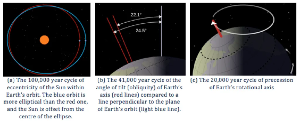
Second, Earth rotates around an axis through the North and South poles, and that axis is at an angle to the plane of Earth’s orbit around the Sun (Figure 16.4b). The angle of tilt (also known as obliquity) varies on a time scale of 41,000 years. When the angle is at its maximum (24.5°), Earth’s seasonal differences are accentuated. When the angle is at its minimum (22.1°), seasonal differences are minimized. The current hypothesis is that glaciation is favoured at low seasonal differences as summers would be cooler and snow would be less likely to melt and more likely to accumulate from year to year.
Third, the direction in which Earth’s rotational axis points also varies, on a time scale of about 20,000 years (Figure 16.4c). This variation, known as precession, means that although the North Pole is presently pointing to the star Polaris (the pole star), in 10,000 years it will point to the star Vega.
The importance of eccentricity, tilt, and precession to Earth’s climate cycles (now known as Milankovitch Cycles) was first pointed out by Yugoslavian engineer and mathematician Milutin Milankovitch in the early 1900s. Milankovitch recognized that although the variations in the orbital cycles did not affect the total amount of insolation (light energy from the Sun, or incoming solar radiation) that Earth received, it did affect where on Earth that energy was strongest. Glaciations are most sensitive to the insolation received at latitudes of around 65°, and with the current configuration of continents, it would have to be 65° N (because there is almost no land at 65° S).
The most important issues are whether the northern hemisphere is pointing toward the sun at its closest or farthest approach, and how eccentric the sun’s position is in Earth’s orbit. Two opposing situations are illustrated in Figure 16.5. In the upper panel, the northern hemisphere is at it farthest distance from the Sun during summer, which means cooler summers. In the lower panel, the northern hemisphere is at its closest distance to the Sun during summer, which means hotter summers. Cool summers — as opposed to cold winters — are the key factor in the accumulation of glacial ice, so the upper scenario in Figure 16.5 is the one that promotes glaciation. This factor is greatest when eccentricity is high.
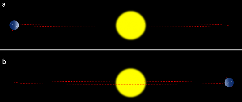
![Figure 19.5 Insolation at 65° N in July compared with Antarctic ice core temperatures [By SE, using data from Valerie Masson-Delmotte, EPICA Dome C ice core 800KYr deuterium data and temperature estimates WDCA Contribution Series Number : 2007 -091 NOAA/NCDC Paleoclimatology Program, Boulder CO, USA. Retrieved from: ftp://ftp.ncdc.noaa.gov/pub/data/paleo/icecore/antarctica/epica_domec/edc3deuttemp2007.txt and from Berger, A. and Loutre, M.F. (1991). Insolation values for the climate of the last 10 million years. Quaternary Science Reviews, 10, 297-317.]](https://openpress.usask.ca/app/uploads/sites/29/2017/05/Insolation-at-65N-in-July.png "Chapter 1. Introduction to Geology")
![Figure 19.6 Variations in the ENSO index from 1950 to 2015 [SE after NOAA at: http://www.esrl.noaa.gov/psd/enso/mei/]](https://openpress.usask.ca/app/uploads/sites/29/2017/05/Variations-in-the-ENSO-index.png "Chapter 1. Introduction to Geology")
Milankovitch Cycles Are Important Because of Climate Feedbacks
As already stated, climate feedbacks are critically important in amplifying weak climate forcings into full-blown climate changes. When Milankovitch published his theory in 1924, it was widely ignored, partly because it was evident to climate scientists that the forcing produced by the orbital variations was not strong enough to drive the significant climate changes of the glacial cycles. Those scientists did not recognize the power of positive feedbacks. It wasn’t until 1973, 15 years after Milankovitch’s death, that sufficiently high-resolution data were available to show that the Pleistocene glaciations were indeed driven by the orbital cycles, and it became evident that the orbital cycles were just the forcing that initiated a range of feedback mechanisms that made the climate change.
Since Earth still has a very large volume of ice — mostly in the continental ice sheets of Antarctica and Greenland, but also in alpine glaciers and permafrost — melting is one of the key feedback mechanisms. Melting of ice and snow leads to several different types of feedbacks, an important one being a change in albedo. Albedo is a measure of the reflectivity of a surface. Earth’s various surfaces have widely differing albedos, expressed as the percentage of light that reflects off a given material. This is important because most solar energy that hits a very reflective surface is not absorbed and therefore does little to warm Earth. Water in the oceans or on a lake is one of the darkest surfaces, reflecting less than 10% of the incident light, while clouds and snow or ice are among the brightest surfaces, reflecting 70% to 90% of the incident light (Figure 16.8).
![Figure 19.7 Typical albedo values for Earth surfaces [SE]](https://openpress.usask.ca/app/uploads/sites/29/2017/05/Typical-albedo-values-for-Earth-surfaces-1024x339.png "Chapter 1. Introduction to Geology")
Exercise 16.2 Albedo Implications of Forest Harvesting

When sea ice melts, as it has done in the Arctic Ocean at a disturbing rate over the past decade, the albedo of the area affected changes dramatically, from around 80% down to less than 10%. Much more solar energy is absorbed by the water than by the pre-existing ice, and the temperature increase is amplified. The same applies to ice and snow on land, but the difference in albedo is not as great.
When ice and snow on land melt, sea level rises. (Sea level is also rising because the oceans are warming and that increases their volume.) A higher sea level means a larger proportion of the planet is covered with water, and since water has a lower albedo than land, more heat is absorbed and the temperature goes up a little more. Since the last glaciation, sea-level rise has been about 125 m; a huge area that used to be land is now flooded by heat-absorbent seawater. During the current period of anthropogenic climate change, sea level has risen only about 20 cm, and although that doesn’t make a big change to albedo, sea-level rise is accelerating.
Most of northern Canada has a layer of permafrost that ranges from a few centimetres to hundreds of metres in thickness; the same applies in Alaska, Russia, and Scandinavia. Permafrost is a mixture of soil and ice (Figure 16.9), and it also contains a significant amount of trapped organic carbon that is released as CO2 and CH4 when the permafrost breaks down. Because the amount of carbon stored in permafrost is in the same order of magnitude as the amount released by burning fossil fuels, this is a feedback mechanism that has the potential to equal or surpass the forcing that has unleashed it.
![Figure 19.8 A degrading permafrost site on the north coast of Alaska [http://alaska.usgs.gov/science/interdisciplinary_science/cae/images/theme2_fig2_lg.jpg]](https://openpress.usask.ca/app/uploads/sites/29/2017/05/degrading-permafrost-site-1024x591.jpg "Chapter 1. Introduction to Geology")
There is about 45 times as much carbon in the ocean (as dissolved bicarbonate ions, HCO3-) as there is in the atmosphere (as CO2), and there is a steady exchange of carbon between the two reservoirs. But the solubility of CO2 in water decreases as the temperature goes up. In other words, the warmer it gets, the more of that oceanic bicarbonate gets transferred to the atmosphere as CO2. That makes CO2 solubility another positive feedback mechanism.
Vegetation growth responds positively to both increased temperatures and elevated CO2 levels, and so in general, it represents a negative feedback to climate change because the more the vegetation grows, the more CO2 is taken from the atmosphere. But it’s not quite that simple because when trees grow bigger and more vigorously, forests become darker (they have lower albedo) so they absorb more heat. Furthermore, climate warming isn’t necessarily good for vegetation growth; some areas have become too hot, too dry, or even too wet to support the plant community that was growing there, and it might take centuries for something to replace it successfully.
All of these positive (and negative) feedbacks work both ways. For example, during climate cooling, growth of glaciers leads to higher albedos, and formation of permafrost results in storage of carbon that would otherwise have returned quickly to the atmosphere.
16.2 Anthropogenic Climate Change
When we talk about anthropogenic climate change, we are generally thinking of the industrial era, which really got going when we started using fossil fuels (coal to begin with) to drive machinery and trains. That was around the middle of the 18th century. The issue with fossil fuels is that they involve burning carbon that was naturally stored in the crust over hundreds of millions of years as part of Earth’s process of counteracting the warming Sun.
Some climate scientists argue that anthropogenic climate change actually goes back much further than the industrial era, and that humans began to impact the climate by clearing land to grow grains in Europe and the Middle East around 8,000 years BCE and by creating wetlands to grow rice in Asia around 5,000 years BCE. Clearing forests for crops is a type of climate-forcing because the CO2 storage capacity of the crops is generally lower than that of the trees they replace, and creating wetlands is a type of climate forcing because the anaerobic bacterial decay of organic matter within wetlands produces CH4.
In fact, whether anthropogenic climate change started with the agricultural revolution or the industrial revolution is not important, because the really significant climate changes didn’t start until the early part of the 20th century, and although our activities are a major part of the problem, our increasing numbers are a big issue as well. Figure 16.10 shows the growth of the world population from around 5 million, when we first started growing crops, to about 18 million when wetland rice cultivation began, to over 800 million at the start of the industrial revolution, to over 7,300 million today. A big part of the incredible growth in our population is related to the availability of the cheap and abundant energy embodied in fossil fuels, which we use for transportation, heating and cooling, industry, and food production. Given that we must support a population of this size, it will be a challenge to convert to non-fossil fuels, but it is doable.
![Figure 19.9 World population growth over the past 12,000 years [by SE from data at: http://ourworldindata.org/roser/graphs/WorldPopulationAnnual12000years_interpolated_HYDEandUN/WorldPopulationAnnual12000years_interpolated_HYDEandUN.csv]](https://openpress.usask.ca/app/uploads/sites/29/2017/05/World-population-growth-over-the-past-12000-years-.png "Chapter 1. Introduction to Geology")
![Figure 19.10 Global mean annual temperatures for the period from 1880 to 2014 [by SE from data at NASA at: http://data.giss.nasa.gov/gistemp/tabledata_v3/GLB.Ts+dSST.txt]](https://openpress.usask.ca/app/uploads/sites/29/2017/05/Global-mean-annual-temperatures.png "Chapter 1. Introduction to Geology")
The Intergovernmental Panel on Climate Change (IPCC), established by the United Nations in 1988, is responsible for reviewing the scientific literature on climate change and issuing periodic reports on several topics, including the scientific basis for understanding climate change, our vulnerability to observed and predicted climate changes, and what we can do to limit climate change and minimize its impacts. Figure 16.12, from the fifth report of the IPCC, issued in 2014, shows the relative contributions of various GHGs and other factors to current climate forcing, based on the changes from levels that existed in 1750. Figure 16.13 shows the IPCC’s projections for temperature increases over the next 100 years.
The biggest anthropogenic contributor to warming is the emission of CO2, which accounts for 50% of positive forcing. CH4 and its atmospheric derivatives (CO2, H2O, and O3) account for 29%, and the halocarbon gases (mostly leaked from air-conditioning appliances) and nitrous oxide (N2O) (from burning fossils fuels) account for 5% each. Carbon monoxide (CO) (also produced by burning fossil fuels) accounts for 7%, and the volatile organic compounds other than methane (NMVOC) account for 3%.
CO2 emissions come mostly from coal- and gas-fired power stations, motorized vehicles (cars, trucks, and aircraft), and industrial operations (e.g., smelting), and indirectly from forestry. CH4 emissions come from production of fossil fuels (escape from coal mining and from gas and oil production), livestock farming (mostly beef), landfills, and wetland rice farming. N2O and CO come mostly from the combustion of fossil fuels. In summary, close to 70% of our current GHG emissions come from fossil fuel production and use, while most of the rest comes from agriculture and landfills.
![Figure 19.11 The relative importance of factors that are contributing to anthropogenic warming [from http://www.ipcc.ch/report/graphics/index.php?t=Assessment%20Reports&r=AR5%20-%20WG1&f=SPM]](https://openpress.usask.ca/app/uploads/sites/29/2017/05/importance-of-factors-that-are-contributing-to-anthropogenic-warming-1024x860.jpg "Chapter 1. Introduction to Geology")
Exercise 16.3 What Does Radiative Forcing Tell Us?
The bottom part of Figure 16.12 shows the total radiative forcing levels for 2011, 1980, and 1950, expressed relative to the forcing that existed in 1750. This forcing is measured in radiance at Earth’s surface in watts per square metre. For reference, the daily average irradiance for Earth is approximately 240 W/m2, so compared with 1750, we’ve increased that by 2.29 W/m2, or a little under 1%.
We can use radiative forcing numbers to estimate the impact on Earth’s surface temperature by applying the following simple equation: ΔT = ΔF * 0.8, where ΔT is the expected change in average surface temperature and ΔF is the change in radiative forcing. Applying this to the value for 2011, we get
ΔT = 0.8 * 2.29 = 1.8°C.
From Figure 16.11, you can see that the global temperature difference between 1880 and 2011 is 0.8 – (-0.6) = 1.4°C. The temperature change between 1750 and 1880 could have been close to 0.4°C, so that puts us in about the right range.
Use the ΔT = ΔF * 0.8 equation to estimate the temperature differences for 1950 and 1980, and see how those compare with the actual temperatures from Figure 16.11.
![Figure 19.12 Projected global temperature increases for the 21st century based on a range of different IPCC scenarios of future political and technological variables [from https://www.ipcc.ch/publications_and_data/ar4/wg1/en/fig/figure-spm-5-l.png]](https://openpress.usask.ca/app/uploads/sites/29/2017/05/Projected-global-temperature-increases-1024x816.png "Chapter 1. Introduction to Geology")
16.3 Implications of Climate Change
We’ve all experienced the effects of climate change over the past decade. However, it’s not straightforward for climatologists to make the connection between a warming climate and specific weather events, and most are justifiably reluctant to ascribe any specific event to climate change. In this respect, the best measures of climate change are those that we can detect over several decades, such as the temperature changes shown in Figure 16.11, or the sea-level rise shown in Figure 16.14. Sea level has risen approximately 20 cm since 1750, and that rise is attributed to both warming (and therefore expanding) seawater and melting glaciers and other land-based snow and ice (melting of sea ice does not contribute directly to sea-level rise as it is already floating in the ocean).
![Figure 19.13 Projected sea-level increases to 2100, showing likely range (grey) and possible maximum [Adapted by SE from: http://nca2014.globalchange.gov/report/our-changing-climate/sea-level-rise#intro-section-2 based on data in Parris et al., 2012, NOAA]](https://openpress.usask.ca/app/uploads/sites/29/2017/05/Projected-sea-level-increases-to-2100.png "Chapter 1. Introduction to Geology")
In a 2008 report, the Organisation for Economic Co-operation and Development (OECD) estimated that by 2070 approximately 150 million people living in coastal areas could be at risk of flooding due to the combined effects of sea-level rise, increased storm intensity, and land subsidence. The assets at risk (buildings, roads, bridges, ports, etc.) are in the order of $35 trillion ($35,000,000,000,000). Countries with the greatest exposure of population to flooding are China, India, Bangladesh, Vietnam, U.S.A., Japan, and Thailand. Some of the major cities at risk include Shanghai, Guangzhou, Mumbai, Kolkata, Dhaka, Ho Chi Minh City, Tokyo, Miami, and New York.
One of the other risks for coastal populations, besides sea-level rise, is that climate warming is also associated with an increase in the intensity of tropical storms (e.g., hurricanes or typhoons), which almost always bring serious flooding from intense rain and storm surges. Some recent examples are New Orleans in 2005 with Hurricane Katrina, and New Jersey and New York in 2012 with Hurricane Sandy (Figure 16.15).
![Figure 19.14 Damage to the Casino Pier, Seaside Heights, New Jersey, from Hurricane Sandy, November 2012 [https://upload.wikimedia.org/wikipedia/commons/c/cb/Hurricane_Sandy_New_Jersey_Pier.jpg]](https://openpress.usask.ca/app/uploads/sites/29/2017/05/Damage-to-the-Casino-Pier-1024x575.jpg "Chapter 1. Introduction to Geology")
![Figure 19.15 Relationship between Atlantic tropical storm cumulative annual intensity and Atlantic sea-surface temperatures [By SE from data at: http://wind.mit.edu/~emanuel/Papers_data_graphics.htm]](https://openpress.usask.ca/app/uploads/sites/29/2017/05/Relationship-between-Atlantic-tropical-storm-cumulative-annual-intensity-and-Atlantic-sea-surface-temperatures-1024x657.png "Chapter 1. Introduction to Geology")
Because warm air is able to hold more water than cold air, the general global trend over the past century has been one of increasing precipitation (Figure 16.17).
![Figure 19.16 Global precipitation anomalies compared with the average over the period from 1901 to 2000 [By NASA, from: http://www.epa.gov/climatechange/science/indicators/weather-climate/precipitation.html]](https://openpress.usask.ca/app/uploads/sites/29/2017/05/Global-precipitation-anomalies.png "Chapter 1. Introduction to Geology")
![Figure 19.17 Change in precipitation amounts over the period 1945 to 2005 for 29 stations in British Columbia [By SE, using data from Environment Canada]](https://openpress.usask.ca/app/uploads/sites/29/2017/05/Change-in-precipitation-amounts-over-the-period-1945-to-2005.png "Chapter 1. Introduction to Geology")
Exercise 16.4 Rainfall and ENSO
This graph shows the monthly precipitation data for Penticton from 1950 to 2005 along with the ENSO (El Niño Southern Oscillation) index values. High ENSO index values correspond to strong El Niño events, such as 1983 and 1998. Describe the relationship between ENSO and precipitation in B.C.’s southern interior. It’s not necessarily a consistent relationship.

The geographical ranges of diseases and pests, especially those caused or transmitted by insects, have been shown to extend toward temperate regions because of climate change. West Nile virus and Lyme disease are two examples that already directly affect Canadians, while dengue fever could be an issue in the future. Canadians are also indirectly affected by the increase in populations of pests such as the mountain pine beetle (Figure 16.19).
![Figure 19.18 Mountain pine beetle damage in Manning Park, British Columbia [https://upload.wikimedia.org/wikipedia/en/7/7c/Pine_Beetle_in_Manning_Park.jpg]](https://openpress.usask.ca/app/uploads/sites/29/2017/05/Mountain-pine-beetle-damage-1024x765.jpg "Chapter 1. Introduction to Geology")
![Figure 19.19 Numbers of various types of disasters between 1971 and 2010 [From WMO atlas of mortality and economic Losses from weather, climate and water extremes, 2014]](https://openpress.usask.ca/app/uploads/sites/29/2017/05/Numbers-of-various-types-of-disasters-between-1971-and-2010.png "Chapter 1. Introduction to Geology")
![Figure 19.20 Temperature anomalies across Russia and neighbouring regions during July 2010 [http://earthobservatory.nasa.gov/IOTD/view.php?id=45069]](https://openpress.usask.ca/app/uploads/sites/29/2017/05/Temperature-anomalies-across-Russia-1024x590.png "Chapter 1. Introduction to Geology")
Exercise 16.5 How Can You Reduce Your Impact on the Climate?
If you look back to Figure 16.12 and the related text, you can easily see what aspects of our way of life are the most responsible for climate change. Think about how you could make changes to your own lifestyle to reduce your impact on the climate. It may depend on where you live, and the degree to which fossil fuels are used to generate the electricity that you use, but it’s most likely to include how, how far, how fast, and how frequently you move around.
If you hold the opinion that there isn’t much point in making changes to your lifestyle because others won’t or because your contribution is only a tiny fraction of the problem, bear in mind that all of us have the opportunity to set an example that others can follow. And remember the words of the American anthropologist Margaret Mead: “Never doubt that a small group of thoughtful, committed citizens can change the world. Indeed, it is the only thing that ever has.”
Chapter 16 Summary
The main topics of this chapter can be summarized as follows:
16.1 What Makes the Climate Change?
The two components of climate change are forcings and feedbacks. Natural climate forcings, which have operated throughout geological time, include solar evolution and cycles, continental drift, continental collisions and mountain building, volcanism, orbital variations, and ocean current cycles. Feedbacks include melting of ice, snow, and permafrost (changing albedo and releasing GHGs); temperature-related changes to solubility of CO2; and vegetation growth.
16.2 Anthropogenic Climate Change
The key contributors to anthropogenic climate change are our use of fossil fuels and our increasing numbers, although other important factors include what we eat and how we produce it.
16.3 Implications of Climate Change
The most reliable indicators of climate change are those that we can detect by looking at records going back for decades. These include temperature and other climate parameters, of course, but also sea-level rise and the incidence of major storms. Some of the implications of climate change include changes to the distribution of disease vectors and pests, and an increase in the incidence and severity of heat waves.
Questions for Review
- What property of greenhouse gases allows them to absorb infrared radiation and thus trap heat within the atmosphere?
- Explain why the emission of CO2 from fossil fuel use is a climate forcing, while the solubility of CO2 in seawater is a climate feedback.
- Explain how the positioning of Gondwana at the South Pole contributed to glaciation during the Paleozoic.
- Most volcanic eruptions lead to short-term cooling, but long-term sustained volcanism can lead to warming. Describe the mechanisms for these two different consequences.
- Using the orbital information on eccentricity, tilt, and precession, we could calculate variations in insolation for any latitude on Earth and for any month of the year. Why is it useful to choose the latitude of 65° as opposed to something like 30°? Why north instead of south? Why July instead of January?
- If the major currents in the oceans were to slow down or stop, how would that affect the distribution of heat on Earth, and what effect might that have on glaciation?
- Explain the climate implications of the melting and breakdown of permafrost.
- Much of the warming of the Paleocene-Eocene thermal maximum is thought to have been caused by the release of CH4 from sea-floor methane hydrates. Describe what would have to have happened before this could take place.
- Burning fossil fuels emits CO2 to the atmosphere via reactions like this one: CH4 + O2 —-> CO2 + 2H2O. Describe some of the other ways that our extraction, transportation, and use of fossil fuels impact the climate.
- Explain why, even if we could stop our impact on the climate tomorrow, we would still be facing between 1 m and 2 m of additional sea-level rise.
- Use the Internet to research West Nile virus, and explain why its spread into Canada from the United States is related to climate change.
10.1 Controls on Metamorphic Processes
The main factors that control metamorphic processes are:
- The mineral composition of the parent rock
- The temperature at which metamorphism takes place
- The amount and type (direction) of pressure during metamorphism
- The amount and type of fluid (mostly water) that is present during metamorphism
- The amount of time available for metamorphism
Parent Rocks Are Changed to Make Metamorphic Rocks
The parent rock or protolith is the rock that exists before metamorphism starts. It can be any of the three rock types: sedimentary, igneous, or metamorphic. The critical feature of the parent rock is its mineral composition. This is because the stability of minerals (how influenced they are by changing conditions) is what counts when metamorphism takes place. In other words, when a rock is subjected to increased temperatures and pressures, certain minerals will undergo chemical reactions and turn into new minerals, while others might just change their shape.
But Which Parent Rock Are You Referring To?
Because some metamorphic rocks form as part of a continuous series as pressures and temperatures increase progressively, some people use the term parent rock to apply to the very first rock that metamorphism happened to, rather than referring to each stage of metamorphic rock as the parent rock to the next stage. The problem is that we won’t always know whether metamorphism happened in an uninterrupted sequence or whether metamorphism stopped and started again for different reasons at different times. If the former is the case it would be no problem to use this system, but if the latter is the case, then it is important to not skip over the intervening steps by saying they are part of a smooth series. For that reason we will use the term parent rock to apply to the direct precursor of the metamorphic rock we’re interested in.
Temperature
The temperature that the rock is subjected to is a key variable in controlling the type of metamorphism that takes place. As we learned in the context of igneous rocks, mineral stability is a function of temperature, pressure, and the presence of fluids (especially water). All minerals are stable over a specific range of temperatures. For example, quartz is stable from surface temperatures (whatever the weather can throw at it) all the way up to about 1800°C. If the pressure is higher, that upper limit will be higher. If there is water present, it will be lower. On the other hand, most clay minerals are only stable up to about 150° or 200°C. Above that, they transform into micas. Most other common minerals have upper limits between 150°C and 1000°C.
Some minerals will crystallize into different polymorphs (same composition but different crystalline structure) depending on the temperature and pressure. Quartz is a good example because slightly different forms are stable between 0°C and 1800°C. The minerals kyanite, andalusite, and sillimanite are polymorphs with the composition Al2SiO5. They are stable at different pressures and temperatures, and, as we will see later, they are important indicators of pressures and temperatures in metamorphic rocks (Figure 10.3).
![Figure 7.3 The temperature and pressure stability fields of the three polymorphs of Al2SiO5. (Pressure is equivalent to depth. Kyanite is stable at low to moderate temperatures and low to high pressures, andalusite at moderate temperatures and low pressures, and sillimanite is stable at higher temperatures.) [SE]](https://openpress.usask.ca/app/uploads/sites/29/2017/05/image0031.png "Chapter 1. Introduction to Geology")
Pressure
Pressure is important in metamorphic processes for two main reasons. First, it has implications for mineral stability (Figure 10.3). Second, it has implications for the texture of metamorphic rocks. Rocks that are subjected to very high confining pressures are typically denser than others because the mineral grains are squeezed together (Figure 10.4a), and because they may contain mineral polymorphs in which the atoms are more closely packed. Because of plate tectonics, pressures within the crust are typically not applied equally in all directions. In areas of plate convergence, the pressure in one direction (perpendicular to the direction of convergence) is typically greater than in the other directions (Figure 10.4b). In situations where different blocks of the crust are being pushed in different directions, the rocks will be subjected to sheer stress (Figure 10.4c).
One of the results of directed pressure and sheer stress is that rocks become foliated — meaning that minerals within them become aligned. Foliation is described in more detail later in this chapter.
![Different types of pressure on rocks. (a) confining pressure, where pressure is essentially equal in all directions, (b) directed pressure, where the pressure form the sides is greater than that from the top and bottom, and (c) sheer stress caused by different blocks of rock being pushed in different directions. [Steven Earle CC-BY 4.0]](https://openpress.usask.ca/app/uploads/sites/29/2017/05/meta_stress.png "Chapter 1. Introduction to Geology")
Fluids
Water is the main fluid present within rocks of the crust, and the only one that we’ll consider here. The presence of water is important for two main reasons. First, water facilitates the transfer of ions between minerals and within minerals, and therefore increases the rates at which metamorphic reactions take place. So, while the water doesn’t necessarily change the outcome of a metamorphic process, it speeds the process up so metamorphism might take place over a shorter time period, or metamorphic processes that might not otherwise have had time to be completed are completed.
Secondly, water, especially hot water, can have elevated concentrations of dissolved substances, and therefore it is an important medium for moving certain elements around within the crust. So not only does water facilitate metamorphic reactions on a grain-to-grain basis, it also allows for the transportation of ions from one place to another. This is very important in hydrothermal processes[footnote]Processes involving water (hydro) and heat (thermal).[/footnote], which are discussed toward the end of this chapter, and in the formation of mineral deposits.
Time
Most metamorphic reactions take place at very slow rates. For example, the growth of new minerals within a rock during metamorphism has been estimated to be about 1 mm per million years. For this reason, it is very difficult to study metamorphic processes in a lab.
While the rate of metamorphism is slow, the tectonic processes that lead to metamorphism are also very slow, so in most cases, the chance for metamorphic reactions to be completed is high. For example, one important metamorphic setting is many kilometres deep within the roots of mountain ranges. A mountain range takes tens of millions of years to form, and tens of millions of years more to be eroded to the extent that we can see the rocks that were metamorphosed deep beneath it.
Exercise 10.1 How Long Did It Take?
 This photo shows a sample of garnet-mica schist from the Greek island of Syros. The large reddish crystals are garnet, and the surrounding light coloured rock is dominated by muscovite mica. The Euro coin is 23 mm in diameter. Assume that the diameters of the garnets increased at a rate of 1 mm per million years.
Based on the approximate average diameter of the garnets visible, estimate how long this metamorphic process might have taken.
[http://commons.wikimedia.org/wiki/File:Garnet_Mica_Schist_Syros_Greece.jpg]
10.2 Classification of Metamorphic Rocks
There are two main types of metamorphic rocks. Foliated metamorphic rocks form under directed pressure (pressure that is not the same in all directions) or shear stress (forces acting parallel to each other, and having the result of “smearing” the rock). Non-foliated rocks form where pressure is uniform, or near the surface with very little pressure at all. Non-foliated metamorphic rocks also form when the parent rock consists of blocky minerals (e.g., quartz, calcite) which can’t be aligned because they aren’t longer in any one dimension.
How Foliation Develops
When a rock is squeezed under directed pressure during metamorphism, this can change the texture such that minerals are elongated in the direction perpendicular to the main stress (Figure 10.5).
![Squeezing during metamorphism causes minerals to stretch out perpendicular to the direction of greatest stress. [SE]](https://openpress.usask.ca/app/uploads/sites/29/2017/05/image006.png "Chapter 1. Introduction to Geology")
![The textural effects of squeezing and aligned mineral growth during metamorphism. The left-hand diagram represents shale with bedding in the direction shown. The right-hand diagram represents schist (derived from that shale), with the mica crystals orientated perpendicular to the main stress direction and the original bedding no longer easily visible. [SE]](https://openpress.usask.ca/app/uploads/sites/29/2017/05/image007.png "Chapter 1. Introduction to Geology")
![A slate boulder on the side of Mt. Wapta in the Rockies near Field, BC. Bedding is visible as light and dark bands sloping steeply to the right (white arrow). Slaty cleavage is evident from the way the rock has broken and also from lines of weakness that same trend (yellow arrows). [SE]](https://openpress.usask.ca/app/uploads/sites/29/2017/05/image008.jpg "Chapter 1. Introduction to Geology")
Most foliation develops when new minerals are forced to grow perpendicular to the direction of greatest stress (Figure 10.6). This effect is especially strong if the new minerals are platy like mica or elongated like amphibole. The mineral crystals don’t have to be large to produce foliation. Slate, for example, is characterized by aligned flakes of mica that are too small to see.
Types of Foliated Metamorphic Rocks
The types of foliated metamorphic rocks, listed in order of metamorphic grade or intensity of metamorphism are slate, phyllite, schist, and gneiss (Figure 10.8). Each of these has a characteristic type of foliation
![Figure 7.8 Examples of foliated metamorphic rocks [a, b and d: SE, c: Michael C. Rygel, http://en.wikipedia.org/wiki/Schist#mediaviewer/File:Schist_detail.jpg]](https://openpress.usask.ca/app/uploads/sites/29/2017/05/foliated-metamorphic-rocks-.png "Chapter 1. Introduction to Geology")
Phyllite is similar to slate, but has typically been heated to a higher temperature. As a result, the micas have grown larger. They still are not visible as individual crystals, but the larger size leads to a satiny sheen on the surface. The cleavage of phyllite is slightly wavy compared to that of slate.
Schist forms at higher temperatures and pressures and has mica crystals which are large enough to see. Other minerals such as garnet might also be visible, but the rock consists predominantly of a single mineral. The cleavage of schist is wavier than that of phyllite.
Gneiss forms at the highest pressures and temperatures, has crystals large enough to see, and has minerals that have separated into bands of different colours. Sometimes the bands are very obvious and continuous, but sometimes they are more like lenses. In the example shown in Figure 10.8d, the dark bands are largely amphibole while the light-coloured bands are feldspar and quartz. Most gneiss has little or no mica because it forms at temperatures higher than those under which micas are stable.
While slate and phyllite typically form only from mudrock, schist and especially gneiss can form from a variety of parent rocks, including mudrock, sandstone, conglomerate, and a range of both volcanic and intrusive igneous rocks.
Schist and gneiss can be named on the basis of important minerals that are present. For example a schist derived from basalt is typically rich in the mineral chlorite, so we call it chlorite schist. One derived from shale may be a muscovite-biotite schist, or just a mica schist, or if there are garnets present it might be mica-garnet schist. Similarly, a gneiss that originated as basalt and is dominated by amphibole, is an amphibole gneiss or amphibolite (Figure 10.9).
![Amphibolite in thin section (2mm field of view), derived from metamorphism of a mafic igneous rock. Green crystals are the amphibole hornblende, and colourless crystals are feldspar. [D.J. Waters, University of Oxford, by permission for educational use http://bit.ly/1T2k8Pm]](https://openpress.usask.ca/app/uploads/sites/29/2017/05/amphibolite_pm20-28-300x225.jpg "Chapter 1. Introduction to Geology")
Types of Non-foliated Metamorphic Rocks
Metamorphic rocks that form under either low-pressure conditions or just confining pressure do not become foliated. In most cases, this is because they are not buried deeply, and the heat for the metamorphism comes from a body of magma that has moved into the upper part of the crust. Metamorphism that happens because of proximity to magma is called contact metamorphism. Some examples of non-foliated metamorphic rocks are marble, quartzite, and hornfels.
Marble is metamorphosed limestone. When it forms, the calcite crystals recrystallize (re-form into larger blocky calcite crystals), and any sedimentary textures and fossils that might have been present are destroyed. If the original limestone is pure calcite, then the marble will be white (as in Figure 10.10). On the other hand, if it has impurities such as clay, silica, or magnesium, the marble could be “marbled” in appearance.
![Marble with visible calcite crystals (left) and an outcrop of banded marble (right) [SE (left) and http://gallery.usgs.gov/images/08_11_2010/a1Uh83Jww6_08_11_2010/large/DSCN2868.JPG (right)]](https://openpress.usask.ca/app/uploads/sites/29/2017/05/Marble-.png "Chapter 1. Introduction to Geology")
Quartzite is metamorphosed sandstone (Figure 10.11). It is dominated by quartz, and in many cases, the original quartz grains of the sandstone are welded together with additional silica. Sandstone often contains some clay minerals, feldspar or lithic fragments, so quartzite can also contain impurities.
![Quartzite from the Rocky Mountains, found in the Bow River at Cochrane, Alberta [SE]](https://openpress.usask.ca/app/uploads/sites/29/2017/05/image016.jpg "Chapter 1. Introduction to Geology")

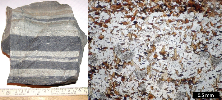
What Happens When Different Rocks Undergo Metamorphism?
As we’ve discussed, the nature of the parent rock controls the types of metamorphic rocks that can form from it under differing metamorphic conditions (temperature, pressure, fluids). The kinds of rocks that can be expected to form at different metamorphic grades from various parent rocks are listed in Table 10.1.
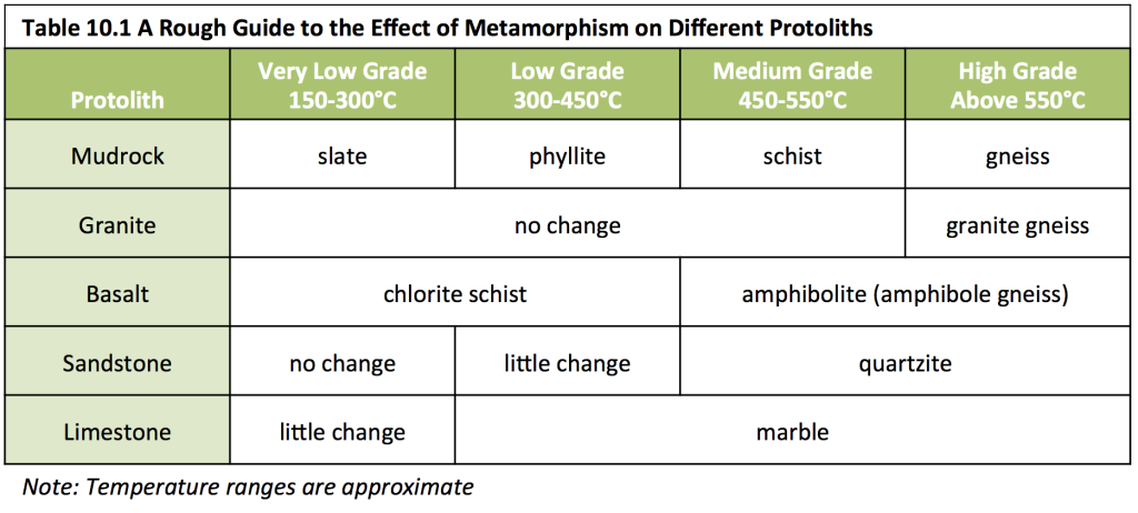
Some rocks, such as granite, do not change much at the lower metamorphic grades because their minerals are still stable up to several hundred degrees. Sandstone and limestone don’t change much either because their metamorphic forms (quartzite and marble, respectively) have the same mineral composition, but re-formed crystals.
On the other hand, some rocks can change substantially. Mudrock (e.g., shale, mudstone) can start out as slate, then progress through phyllite, schist, and gneiss. Schist and gneiss can also form from sandstone, conglomerate, and a range of both volcanic and intrusive igneous rocks.
Migmatite: Not Quite Metamorphic, Not Quite Igneous
If a metamorphic rock is heated enough, it can begin to undergo partial melting in the same way that igneous rocks do. The more felsic minerals (feldspar, quartz) will melt, while the darker minerals (biotite, hornblende) do not. When the melt crystallizes again, the result is light-coloured igneous rock interspersed with dark metamorphic rock. This mixed rock is called migmatite[footnote]Migma is from the ancient Greek for mixture.[/footnote] (Figure 10.14).

![Ptygmatic folding from Broken Hill, New South Wales, Australia. Ptygmatic folding happens when a stiff layer within a rock is surrounded by weaker layers. Folding causes the stiff layer to crinkle while the weaker layers deform around it. [Photo by Roberto Weinberg http://users.monash.edu.au/~weinberg]](https://openpress.usask.ca/app/uploads/sites/29/2017/05/ptygmatic-fold-300x216.jpg "Chapter 1. Introduction to Geology")
![Sketch of a microscopic view of a ptygmatic fold after Hollocher (2014). Field of view is approximately 2 mm. Notice that the mineral crystals (green) are aligned with the axis of the fold (marked with the dashed line) near the fold, but further away they are horizontal, like the solid black line. [KP]](https://openpress.usask.ca/app/uploads/sites/29/2017/05/ptygmatic-fold-ts-300x205.png "Chapter 1. Introduction to Geology")
Exercise 10.2 Naming Metamorphic Rocks
Which metamorphic rock is described in each of the following?
- A rock with visible minerals of mica and with small crystals of andalusite. The mica crystals are consistently parallel to one another.
- A very hard rock with a granular appearance and a glassy lustre. There is no evidence of foliation.
- A fine-grained rock that splits into wavy sheets. The surfaces of the sheets have a sheen to them.
- A rock that is dominated by aligned crystals of amphibole.
10.3 Types of Metamorphism and Where They Occur
The outcome of metamorphism depends on pressure, temperature, and the abundance of fluid involved, and there are a great many settings with unique combinations of these factors. Some types of metamorphism are characteristic of specific plate tectonic settings, but others are not.
Burial Metamorphism
Burial metamorphism occurs when sediments are buried deeply enough that the heat and pressure cause minerals to begin to recrystallize and new minerals to grow, but does not leave the rock with a foliated appearance. As far as metamorphic processes go, burial metamorphism takes place at relatively low temperatures (above 300 °C) and pressures (100s of metres depth). One rock that can form in this setting is metaconglomerate (Figure 10.17). It looks like a regular conglomerate, except the clasts have become elongated.
![A metaconglomerate, displaying clasts that have become elongated. [R. Weller/ Cochise College, by permission for educational use]](https://openpress.usask.ca/app/uploads/sites/29/2017/05/6stretch-pebble-conglomerate3685-300x195.jpg "Chapter 1. Introduction to Geology")
Regional Metamorphism
Regional metamorphism refers to the large-scale metamorphism that happens to continental crust along convergent tectonic margins (where plates collide). The collisions result in the formation of long mountain ranges, like those along the western coast of North America. The force of the collision causes rocks to be folded, and broken and stacked on each other, so not only is there the squeezing force from the collision, but the lithostatic pressure from the weight of rocks being stacked on top of each other. The deeper rocks are within the stack, the higher the pressures and temperatures, and the higher the grade of metamorphism that occurs. Rocks that form from regional metamorphism are likely to be foliated because of the strong directional pressure of converging plates.
The Himalaya range is an example of where regional metamorphism is happening because two continents are colliding (Figure 10.18). Sedimentary rocks have been both thrust up to great heights (nearly 9,000 m above sea level) and also buried to great depths. Considering that the normal geothermal gradient (the rate of increase in temperature with depth) is around 30°C per kilometre in the crust, rock buried to 9 km below sea level in this situation could be close to 18 km below the surface of the ground, and it is reasonable to expect temperatures up to 500°C. In Figure 10.17 the dashed lines are isotherms– lines of equal temperature[footnote]Iso means same, and therm refers to heat.[/footnote]- resulting from the geothermal gradient. Notice the sequence of rocks that from, beginning with slate higher up where pressures and temperatures are lower, and ending in migmatite at the bottom where temperatures are so high that some of the minerals start to melt. These rocks are all foliated, and that is to be expected because of the strong compressing force of the converging plates.
![Figure 7.15 a: Regional metamorphism beneath a mountain range related to continent-continent collision (typical geothermal gradient). (Example: Himalayan Range) [SE]](https://openpress.usask.ca/app/uploads/sites/29/2017/05/image020.png "Chapter 1. Introduction to Geology")
Seafloor (Hydrothermal) Metamorphism
At an oceanic spreading ridge, recently formed oceanic crust of gabbro and basalt is slowly moving away from the plate boundary (Figure 10.19). Water within the crust is forced to rise in the area close to the source of volcanic heat, and this draws more water in from farther out, which eventually creates a convective system where cold seawater is drawn into the crust, heated to 200° to 300°C as it passes through the ocean crust, and released again onto the sea floor near the ridge.
![Hydrothermal metamorphism of oceanic crustal rock on either side of a spreading ridge. (Example: Juan de Fuca spreading ridge) [SE]](https://openpress.usask.ca/app/uploads/sites/29/2017/05/image021.png "Chapter 1. Introduction to Geology")
![Figure 10.19 [http://bit.ly/1Te37Cg]](https://openpress.usask.ca/app/uploads/sites/29/2017/05/800px-Archean_Greenstone_Pillow_Lava_in_Michigan_USA_3-300x188.jpg "Chapter 1. Introduction to Geology")
Subduction Zone Metamorphism
At subuction zones, where oceanic crust is forced down into the hot mantle, there is a unique combination of relatively low temperatures and very high pressures. The high pressures are to be expected, given the force of collision between tectonic plates, and the increasing lithostatic pressure as the subducting slab is forced further and further into the mantle. The lower temperatures exist because even though the mantle is very hot, the ocean crust is relatively cool, and doesn’t take in heat from the mantle rapidly. That means it can be several hundreds of degrees cooler than the surrounding mantle. In Figure 10.21, notice that the isotherms (dotted lines) plunge deep into the mantle along with the subducting slab. This means that regions of relatively low temperature exist deeper in the mantle.
![Figure 7.17 c: Regional metamorphism of oceanic crust at a subduction zone. (Example: Cascadia subduction zone. Rock of this type is exposed in the San Francisco area.) [SE]](https://openpress.usask.ca/app/uploads/sites/29/2017/05/image022.png "Chapter 1. Introduction to Geology")
If you’ve never seen or even heard of blueschist, that not surprising. What is surprising is that anyone has seen it! Most of the blueschist that forms in subduction zones continues to be subducted. It turns into eclogite at about 35 km depth, and then eventually sinks deep into the mantle, never to be seen again. In only a few places in the world, the subduction process was interrupted, and partially subducted blueschist rock returned to the surface. One such place is the area around San Francisco. The blueschist is part of a set of rocks known as the Franciscan Complex (Figure 10.22).
![Figure 7.18 Franciscan Complex blueschist rock exposed north of San Francisco. The blue colour of rock is due to the presence of the amphibole mineral glaucophane. [SE]](https://openpress.usask.ca/app/uploads/sites/29/2017/05/Franciscan-Complex-.png "Chapter 1. Introduction to Geology")
Contact Metamorphism
Contact metamorphism happens when a body of magma intrudes into the upper part of the crust. Heat is important in contact metamorphism, but pressure is not a key factor, so contact metamorphism produces non-foliated metamorphic rocks such as hornfels, marble, and quartzite.
Any type of magma body can lead to contact metamorphism, from a thin dyke to a large stock. The type and intensity of the metamorphism, and width of the metamorphic aureole will depend on a number of factors, including the type of country rock, the temperature of the intruding body and the size of the body (Figure 10.23). A large intrusion will contain more thermal energy and will cool much more slowly than a small one, and therefore will provide a longer time and more heat for metamorphism. That will allow the heat to extend farther into the country rock, creating a larger aureole.
![chematic cross-section of the middle and upper crust showing two magma bodies. The upper body, which has intruded into cool unmetamorphosed rock, has created a zone of contact metamorphism. The lower body is surrounded by rock that is already hot (and probably already metamorphosed), and so it does not have a significant metamorphic aureole. [SE]](https://openpress.usask.ca/app/uploads/sites/29/2017/05/image032-290x300.png "Chapter 1. Introduction to Geology")
Although bodies of magma can form in a variety of settings, one place magma is produced in abundance, and where contact metamorphism can take place, is along convergent boundaries with subduction zones, where volcanic arcs form (Figure 10.24). Regional metamorphism also takes place in this setting, and because of the extra heat associated with the volcanism, the geothermal gradient is typically a little steeper in these settings (somewhere between 40° and 50°C/km). That means higher grades of metamorphism can take place closer to surface than is the case in other areas (note the foliated metamorphic rocks listed on the right-hand side of the diagram).
![Figure 7.19 d: Contact metamorphism around a high-level crustal magma chamber. (Example: the magma chamber beneath Mt. St. Helens.) e: Regional metamorphism in a volcanic-arc related mountain range. (volcanic-region temperature gradient) (Example: The southern part of the Coast Range, BC.) [SE]](https://openpress.usask.ca/app/uploads/sites/29/2017/05/image025.png "Chapter 1. Introduction to Geology")
Shock Metamorphism
When extraterrestrial objects such as meteorites and asteroids hit the Earth, the result is a shock wave. Where the object hits, pressures and temperatures become very high in a fraction of a second. A “gentle” impact can hit with 40 GPa and raise temperatures to up to 500 °C.[footnote]French, B.M. (1998). Impact Melts. (pp. 79-96) In Traces of Catastrophe: A Handbook of Shock-Metamorphic Effects in Terrestrial Meteorite Impact Structures. Houston: Lunar and Planetary Institute http://bit.ly/1LOdapy[/footnote] Pressures in the lower mantle start at 24 GPa (giga Pascals), or and climb to 136 GPa at the core-mantle boundary, so the impact is like plunging the rock deep into the mantle and releasing it again within seconds. The sudden change associated with shock metamorphism makes it very different from other types of metamorphism which can develop over hundreds of millions of years, starting and stopping as tectonic conditions change.
Two features of shock metamorphism are shocked quartz, and shatter cones. Shocked quartz (Figure 10.25 left) refers to quartz crystals which display damage that shows up as parallel lines throughout the crystal. The quartz crystal in Figure 10.25 has two sets of these lines. The lines are small amounts of glassy material within the quartz. Shatter cones are cone-shaped fractures within the rocks (Figure 10.25 right). The fractures are nested together like a stack of ice-cream cones, and point in the direction of the impact.
![Shock metamorphism features. Left: Shocked quartz displaying lines of glassy material, from the Suvasvesi South impact structure in Finland. [Martin Schmieder CC-BY http://bit.ly/24vRcmM] Right: Shatter cones from the Wells Creek impact crater in the USA. [Zamphuor, publc domain http://bit.ly/1n8VBKn]](https://openpress.usask.ca/app/uploads/sites/29/2017/05/impact-meta.png "Chapter 1. Introduction to Geology")
10.4 Metamorphic Facies and Index Minerals
Metamorphic Facies
In any given metamorphic setting there can be a variety of parent-rock types exposed to metamorphism. While these rocks will be exposed to the same range of pressures and temperatures, the metamorphic rock that results will depend on the parent rock. A convenient way to indicate the range of possible metamorphic rocks in a particular setting is to group those possibilities into metamorphic facies[footnote]Facies is a Latin word meaning form, appearance, or face, and in geology it is used to specify a group of rocks. Sedimentary facies, for example, group all the sedimentary rocks that form in a particular depositional environment.[/footnote]. In other words, a given metamorphic facies groups together metamorphic rocks that form under the same pressure and temperature conditions, but which have different protoliths.
Figure 10.26 shows the different metamorphic facies as patches of different colours. The axes on the diagram are temperature and depth; the depth within the Earth will determine how much pressure a rock is under, so the vertical depth axis is also a pressure axis. Therefore, each patch of colour represents a range of temperatures and pressures where particular types of metamorphic rocks will form. The metamorphic facies are named after rocks which form under those particular conditions (e.g., eclogite facies, greenschist facies, amphibolite facies etc.), but those names don’t mean that the facies is limited to that one rock type.

In the context of these diagrams, the yellow, green, and blue dashed lines tell you what metamorphic facies you will encounter for rocks from a given depth in that particular environment. A depth of 15 km in a volcanic region falls in the amphibolite facies. Under more typical conditions, this is the greenschist facies, and in a subduction zone it is the blueschist facies. You can make the connection more directly between the metamorphic facies and the types of metamorphism discussed in the previous section. Notice the letters a through e in Figure 10.26. These match up with the labels in Figure 10.27 below, and can also be found in Figures 10.18, 10.19, 10.21, and 10.24 in the previous section.
![Environments of metamorphism in the context of plate tectonics: (a) regional metamorphism related to mountain building at a continent-continent convergent boundary, (b) seafloor (hydrothermal) metamorphism of oceanic crust in the area on either side of a spreading ridge, (c) metamorphism of oceanic crustal rocks within a subduction zone, (d) contact metamorphism adjacent to a magma body at a high level in the crust, and (e) regional metamorphism related to mountain building at a convergent boundary. [SE]](https://openpress.usask.ca/app/uploads/sites/29/2017/05/image019-1024x300.png "Chapter 1. Introduction to Geology")
Exercise 10.3 Metamorphic Rocks in Areas with Higher Geothermal Gradients
Figure 10.26 shows the types of rock that might form from mudrock at various points along the curve of the “typical” geothermal gradient (dotted green line). Looking at the geothermal gradient for volcanic regions (dotted yellow line in Figure 10.26), estimate the depths at which you would expect to find the same types of rock forming from a mudrock parent.
| Metamorphic Rock Type | Depth (km) |
| Slate | |
| Phyllite | |
| Schist | |
| Gneiss | |
| Migmatite |
Index Minerals
Some common minerals in metamorphic rocks are shown in Figure 10.28, arranged in order of the temperature ranges within which they tend to be stable. The upper and lower limits of the ranges are intentionally vague because these limits depend on a number of different factors, such as the pressure, the amount of water present, and the overall composition of the rock. Even though the limits of the stability ranges are vague, the stability range of each mineral is still small enough that the minerals can be used as markers for those metamorphic conditions. Minerals which make good markers of specific ranges of metamorphic conditions are called index minerals. When geologists are examining the metamorphic rocks in a region, they can use the index minerals to map out zones that experienced different pressures and temperatures.
![Metamorphic index minerals and their approximate temperature ranges [SE]](https://openpress.usask.ca/app/uploads/sites/29/2017/05/image027.png "Chapter 1. Introduction to Geology")
The Meguma Terrane of Nova Scotia: An Example of How to Use Index Minerals
The southern and southwestern parts of Nova Scotia were regionally metamorphosed during the Devonian Acadian Orogeny (around 400 Ma), when a relatively small continental block (the Meguma Terrane[footnote]No, it’s not a spelling mistake! A terrane is a distinctive block of crust that is now part of a continent, but is thought to have come from elsewhere, and was added on by plate-tectonic processes.[/footnote]) was pushed up against the existing eastern margin of North America. The clastic sedimentary rocks within this terrane were variably metamorphosed. Figure 10.29 is a map of zones where different index minerals can be found. This allows us to see where metamorphism was stronger or weaker.

A probable explanation for this pattern is that the area with the highest-grade rocks was buried beneath the central part of a mountain range formed by the collision of the Meguma Terrane with North America. As is the case with all mountain ranges, the crust became thickened as the mountains grew, and it was pushed farther down into the mantle than the surrounding crust. This happens because Earth’s crust is floating on the underlying mantle. As the formation of mountains adds weight, the crust in that area sinks farther down into the mantle to compensate for the added weight. The likely pattern of metamorphism in this situation is shown in cross-section in Figure 10.30a. The mountains were eventually eroded (over tens of millions of years), allowing the crust to rebound upward and exposing the metamorphic rock (Figure 10.30b).


Building a narrative for the metamorphism in Nova Scotia’s Meguma Terrane is just one example of how index minerals can be used.
Exercise 10.4 Scottish Metamorphic Zones
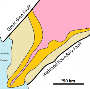
The map shown here represents the part of western Scotland between the Great Glen Fault and the Highland Boundary Fault. The shaded areas are metamorphic rock, and the three metamorphic zones represented are garnet, chlorite, and biotite.
Label the three coloured areas of the map with the appropriate zone names (garnet, chlorite, and biotite).
Indicate which part of the region was likely to have been buried the deepest during metamorphism.
British Geologist George Barrow studied this area in the 1890s and was the first person anywhere to map metamorphic zones based on their mineral assemblages. This pattern of metamorphism is sometimes referred to as “Barrovian.”
10.5 Metamorphic Hydrothermal Processes and Metasomatism
A hot body of magma in the upper crust can create a very dynamic situation that may have geologically interesting and economically important implications. In the simplest cases, water does not play a big role, and the main process is transfer of heat from the pluton to the surrounding rock, creating a zone of contact metamorphism (Figure 10.31a). In many cases, however, water is released from the magma body as crystallization takes place, and this water is dispersed along fractures in the country rock (Figure 10.31b). The water released from a magma chamber is typically rich in dissolved minerals. As this water cools, is chemically changed by the surrounding rocks, or boils because of a drop in pressure, minerals are deposited, forming veins within the fractures in the country rock. Quartz veins are common in this situation, and they might also include pyrite, hematite, calcite, and even silver and gold.
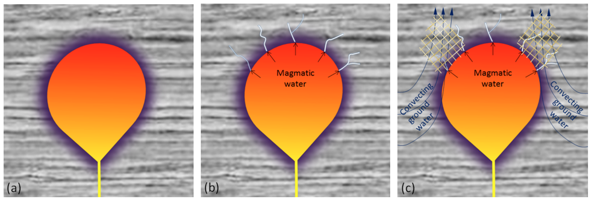
(a) Thermal metamorphism only (within the purple zone)
(b) Thermal metamorphism plus veining (white) related to dispersal of magmatic fluids into the overlying rock
(c) Thermal metamorphism plus veining from magmatic fluids plus alteration and possible formation of metallic minerals (hatched yellow areas) from convection of groundwater
Heat from the magma body will cause surrounding groundwater to expand and then rise toward the surface. In some cases, this may initiate a convection system where groundwater circulates past the pluton. Such a system could operate for thousands of years, resulting in the circulation of millions of tonnes of groundwater from the surrounding region past the pluton.
Hot water circulating through the rocks can lead to significant changes in the mineralogy of the rock, including alteration of feldspars to clays, and deposition of quartz, calcite, and other minerals in fractures and other open spaces (Figure 10.32). As with the magmatic fluids, the nature of this circulating groundwater can also change adjacent to, or above, the pluton, resulting in deposition of other minerals, including ore minerals. Metamorphism in which much of the change is derived from fluids passing through the rock is known as metasomatism. When hot water contributes to changes in rocks, including mineral alteration and formation of veins, it is known as hydrothermal alteration.
![Calcite veins in limestone of the Comox Formation, Nanaimo, BC [SE]](https://openpress.usask.ca/app/uploads/sites/29/2017/05/image036-1024x640.jpg "Chapter 1. Introduction to Geology")
A special type of metasomatism takes place where a hot pluton intrudes into carbonate rock such as limestone. When magmatic fluids rich in silica, calcium, magnesium, iron, and other elements flow through the carbonate rock, their chemistry can change dramatically, resulting in the deposition of minerals that would not normally exist in either the igneous rock or limestone. These include garnet, epidote (another silicate), magnetite, pyroxene, and a variety of copper and other minerals (Figure 10.33). This type of metamorphism is known as skarn.
![A skarn rock from Mount Monzoni, Northern Italy, with recrystallized calcite (blue) garnet (brown) and pyroxene (green). The rock is 6 cm across. [by Siim Sepp, from http://commons.wikimedia.org/wiki/File:00031_6_cm_grossular_calcite_augite_skarn.jpg]](https://openpress.usask.ca/app/uploads/sites/29/2017/05/image037.jpg "Chapter 1. Introduction to Geology")
Exercise 10.5 Contact Metamorphism and Metasomatism
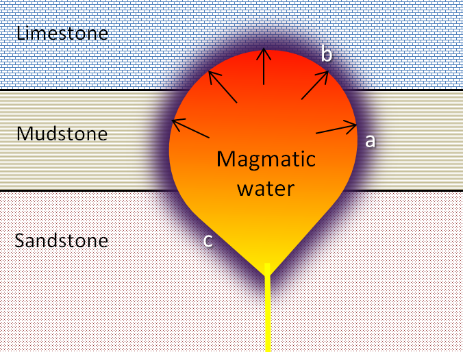
This diagram shows a pluton that has intruded into a series of sedimentary rocks.
What type of metamorphic rock would you expect to see at each location: a, b, and c?
Chapter 10 Summary
The topics covered in this chapter can be summarized as follows:
10.1 Controls on Metamorphic Processes
Metamorphism is controlled by five main factors: the composition of the parent rock, the temperature to which the rock is heated, the amount and type of pressure, the volumes and compositions of aqueous fluids that are present, and the amount of time available for metamorphic reactions to take place.
10.2 Classification of Metamorphic Rocks
Metamorphic rocks are classified on the basis of texture and mineral composition. Foliation is a key feature of metamorphic rocks formed under directed pressure; foliated metamorphic rocks include slate, phyllite, schist, and gneiss. Metamorphic rocks formed in environments without strong directed pressure include hornfels, marble, and quartzite.
10.3 Types of Metamorphism and Where They Occur
Almost all metamorphism can be explained by plate-tectonic processes. Oceanic crustal rock can be metamorphosed near the spreading ridge where it was formed, and regional metamorphism takes place in areas where mountain ranges have formed, which are most common at convergent boundaries. Contact metamorphism takes place around magma bodies in the upper part of the crust, which are also most common above convergent boundaries. Shock metamorphism happens when extraterrestrial bodies impact the Earth, and is a unique metamorphic process in terms of its speed.
10.4 Metamorphic Facies and Index Minerals
Metamorphic facies are a way to group metamorphic rocks which form under the same range of pressure and temperature conditions, but from different parent rocks. Geologists classify metamorphic rocks based on some key minerals — such as chlorite, garnet, andalusite, and sillimanite — and these can tell us about the pressure and temperature conditions under which the rocks formed.
10.5 Metamorphic Hydrothermal Processes and Metasomatism
Contact metamorphism takes place around magma bodies that have intruded into cool rocks at high levels in the crust. Heat from the magma is transferred to the surrounding country rock, resulting in mineralogical and textural changes. Water from a cooling body of magma, or from convection of groundwater produced by the heat of the pluton, can also lead to metasomatism, hydrothermal alteration, and accumulation of valuable minerals in the surrounding rocks.
Questions for Review
- What are the two main agents of metamorphism, and what are their respective roles in producing metamorphic rocks?
- Into what metamorphic rocks will a mudrock be transformed at very low, low, medium, and high metamorphic grades?
- Why doesn’t granite change very much at lower metamorphic grades?
- Describe the main process of foliation development in a metamorphic rock such as schist.
- What process contributes to metamorphism of oceanic crust at a spreading ridge?
- How do variations in the geothermal gradient affect the depth at which different metamorphic rocks form?
- Blueschist metamorphism takes place within subduction zones. What are the particular temperature and pressure characteristics of this geological setting?
- Rearrange the following minerals in order of increasing metamorphic grade: biotite, garnet, sillimanite, chlorite.
- Why does contact metamorphism not normally take place at significant depth in the crust?
- What is the role of magmatic fluids in metamorphism that takes place adjacent to a pluton?
- How does metasomatism differ from regional metamorphism?
- How does the presence of a hot pluton contribute to the circulation of groundwater that facilitates metasomatism and hydrothermal processes?
- What must be present in the country rock to produce a skarn?
- Two things that a geologist first considers when looking at a metamorphic rock are what the parent rock might have been, and what type of metamorphism has taken place. This can be difficult to do, even if you have the actual rock in your hand, but give it a try for the following:
| Metamorphic Rock | Likely Parent Rock | Grade and/or Type of Metamorphism |
| Chlorite schist | ||
| Slate | ||
| Mica-garnet schist | ||
| Amphibolite | ||
| Marble |
4.1 Alfred Wegener — the Father of Plate Tectonics
Alfred Wegener (1880-1930) (Figure 4.1) earned a PhD in astronomy at the University of Berlin in 1904, but he had always been interested in geophysics and meteorology, and spent most of his academic career working in meteorology.
![Alfred Wegener during a 1912-1913 expedition to Greenland. [Source: Alfred Wegener Institute (Public domain)]](https://openpress.usask.ca/app/uploads/sites/29/2017/05/Wegener_Expedition-1930_008.jpg "Chapter 1. Introduction to Geology")
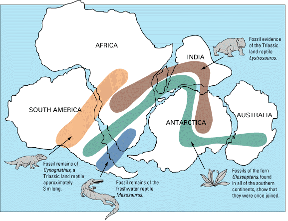
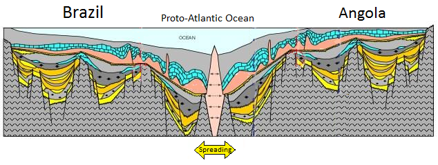
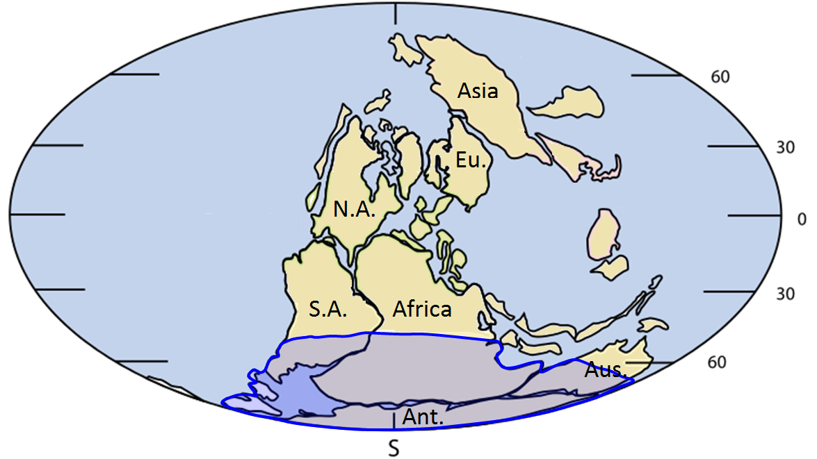
The main problem standing in the way of Wegener’s idea being accepted was that he could not explain how the continents could move around. Remember that, as far as anyone was concerned, the Earth’s crust was continuous, not broken into plates. That means any mechanism Wegener could think of would have to fit with that model of Earth’s structure. Geologists at the time were aware that the continents were made of different rocks than the ocean crust, and that the material making up the continents was less dense, so Wegener proposed that the continents were like icebergs floating on the heavier ocean crust. He suggested that the continents were moved by the effect of Earth’s rotation pushing objects toward the equator, and by the lunar and solar tidal forces, which tend to push objects toward the west. However, it was quickly shown that these forces were far too weak to move continents, and without any reasonable mechanism to make it work, Wegener’s theory was quickly dismissed by most geologists of the day.
Alfred Wegener died in Greenland in 1930 while carrying out studies related to glaciation and climate. At the time of his death, his ideas were tentatively accepted by a small minority of geologists, and firmly rejected by most. However, within a few decades that was all to change. For more about his extremely important contributions to Earth science, visit this NASA website: http://earthobservatory.nasa.gov/Library/Giants/Wegener/
4.2 Global Geological Models of the Early 20th Century
The untimely death of Alfred Wegener didn’t solve any problems for those who opposed his ideas because they still had some inconvenient geological truths to deal with. One of those was explaining the distribution of terrestrial species across five continents that are currently separated by hundreds or thousands of kilometres of ocean water (Figure 4.2), and another was explaining the origin of extensive fold-belt mountains, such as the Appalachians, the Alps, the Himalayas, and the Canadian Rockies.
Before we go any further, it is important to know what was generally believed about global geology before plate tectonics. At the beginning of the 20th century, geologists had a good understanding of how most rocks were formed and understood their relative ages through interpretation of fossils, but there was considerable controversy regarding the origin of mountain chains, especially fold-belt mountains. At the end of the 19th century, one of the prevailing views on the origin of mountains was the theory of contractionism — the idea that since Earth is slowly cooling, it must also be shrinking. In this scenario, mountain ranges had formed like the wrinkles on a dried-up apple, and the oceans had submerged parts of former continents. While this hypothesis helped to address the dilemma of the terrestrial fossils, it came with its own set of problems. One problem was that Earth wasn’t cooling fast enough to create the necessary amount of shrinking. Another problem was the principle of isostasy (which had already been around for several decades), which wouldn’t allow continents to sink. (See Section 3.5 for a review of the important principle of isostasy.)
Another widely held view was permanentism, the idea that the continents and oceans have always been generally as they are today. This view incorporated a mechanism for creation of mountain chains known as the geosyncline theory. A geosyncline is a thick (potentially 1000s of metres) deposit of sediments and sedimentary rocks, typically situated along the edge of a continent, and derived from continental weathering (Figure 4.5).
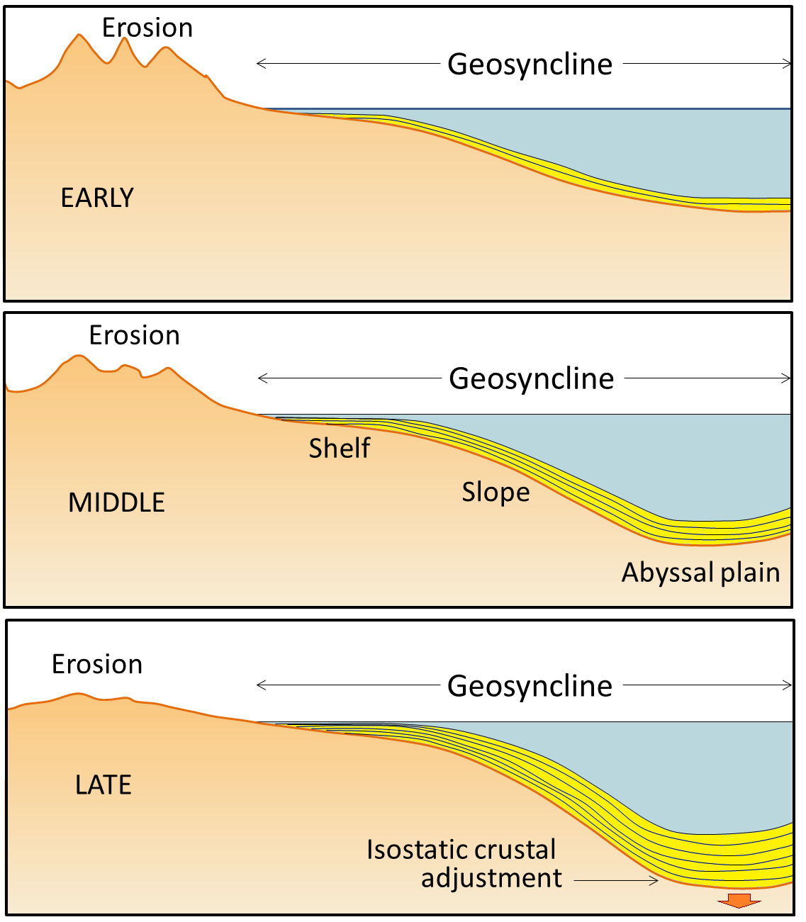
The idea of geosynclines developing into fold-belt mountains originated in the middle of the 19th century, proposed first by James Hall and later elaborated by Dwight Dana, both of whom worked extensively in the Appalachian Mountains of the eastern United States. The process of converting a geosyncline into a mountain belt was never really adequately explained, although it was widely believed that mountain belts formed when geosynclines were compressed by forces pushing from either side. The problem is that, without the lateral forces related to plate tectonics, no one was able to adequately describe what would do the pushing.
Proponents of the geosyncline theory of mountain formation- and there were many well into the 1960s- also had the problem of explaining the intercontinental terrestrial fossil matchups. The simple explanation was that there were “land bridges” across the Atlantic along which animals and plants could migrate back and forth. One proponent of this idea was the American naturalist Ernest Ingersoll. Referring to evidence of past climate changes, Ingersoll contributed the following to the Encyclopedia Americana in 1920: “The most interesting feature of these changes, however, is that by which, now and again, the Old World was connected with the New by necks or spaces of land, known as “land-bridges”; especially as these permitted an interchange of plants and animals, giving to us many new ones from the other side of the ocean, including, finally, man himself.”[footnote]http://en.wikisource.org/wiki/The_Encyclopedia_Americana_(1920)/Land-Bridges_Across_the_Oceans[/footnote]
There are many problems with the land-bridge theory, including the fact that it is inconsistent with isostasy, and that there is no evidence of the remnants of the land bridges. The Atlantic Ocean is several thousand metres deep over wide areas, and so the underwater slopes leading up to a land bridge would have to have been at least tens of kilometres wide in most places, and many times that in others. A land bridge of that size would certainly have left some trace.
Exercise 4.1 Fitting the continents together
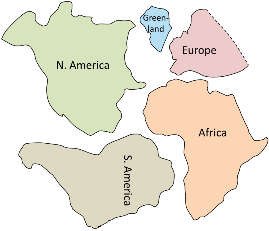
The main continents around the Atlantic Ocean are depicted here in the shapes that they might have had during the Mesozoic, including the extents of their continental shelves. Cut these shapes out and see how well you can fit them together in the positions that these areas occupied within Pangea. You can refer to a map of Pangea to help you make the fit.
4.3 Geological Renaissance of the Mid-20th Century
Two key areas of research ultimately led to the acceptance of continental drift, and the formulation of plate tectonic theory. One was the study of paleomagnetism, the record of Earth’s magnetic field through time. The other was exploration of the ocean floor.
Paleomagnetism (Remnant Magnetism)
![igure 4.6 Rock layers recording remnant magnetism. The red arrows represent the direction of the vertical component of Earth's magnetic field. The oldest rock has a magnetic dip characteristic of the southern hemisphere, but over time the dip changes, indicating that the rocks moved toward magnetic north. [SE]](https://openpress.usask.ca/app/uploads/sites/29/2017/05/image0151.png "Chapter 1. Introduction to Geology")
Rocks like basalt, which cool from a high temperature and commonly have relatively high levels of magnetite, are particularly susceptible to being magnetized in this way. However, even sediments and sedimentary rocks can take on remnant magnetism as long as they have small amounts of magnetic minerals, because the magnetic grains can gradually become lined up with Earth’s magnetic field as the sediments are deposited.
By studying both the horizontal and vertical components of the remnant magnetism, one can tell not only the direction to magnetic north at the time of the rock’s formation, but also the latitude where the rock formed relative to magnetic north. Remember that the vertical component of the magnetic field points more sharply downward the closer it is to the magnetic north pole. Figure 4.6 shows the vertical component of remnant magnetism in a sequence of rocks. Notice that the arrow starts out at 500 Ma pointing slightly upward. This means that the rocks were in the southern hemisphere. As the rocks get younger, the arrow tilts toward horizontal, and then points downward. This indicates that the rocks were getting progressively closer to the north magnetic pole.
Apparent Polar Wandering Paths
In the early 1950s, a group of geologists from Cambridge University, including Keith Runcorn, Ted Irving,[footnote]Ted Irving later set up a paleomagnetic lab at the Geological Survey of Canada in Sidney, B.C., and did a great deal of important work on understanding the geology of western North America.[/footnote] and several others, started looking at the remnant magnetism of Phanerozoic British and European volcanic rocks, and collecting paleomagnetic data. Using an analysis similar to that in Figure 4.6, they noticed that rocks of different ages sampled from the same general area showed very different magnetic pole positions (the green line in Figure 4.7). They assumed this meant that Earth’s magnetic pole had moved around significantly over time along polar wandering paths, rather than staying close to the geographic north pole as it does today. At the time, geophysical models suggested that the magnetic poles did not need to be aligned with the rotational poles, so this wasn’t an unreasonable conclusion, given what was known.
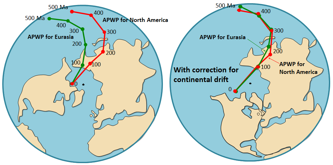
This paleomagnetic work of the 1950s was the first new evidence in favour of continental drift, and it led a number of geologists to start thinking that the idea might have some merit. Nevertheless, for a majority of geologists, this type of evidence was not sufficiently convincing to get them to change their views.
Ocean basin geology and geography
During the 20th century, our knowledge and understanding of the ocean basins and their geology increased dramatically. Before 1900, we knew virtually nothing about the bathymetry (the hills and valleys of the ocean floor) and geology of the oceans. By the end of the 1960s, we had detailed maps of the topography of the ocean floors, a clear picture of the geology of ocean floor sediments and the solid rocks underneath them, and almost as much information about the geophysical nature of ocean rocks as of continental rocks.
Acoustic Depth Sounding
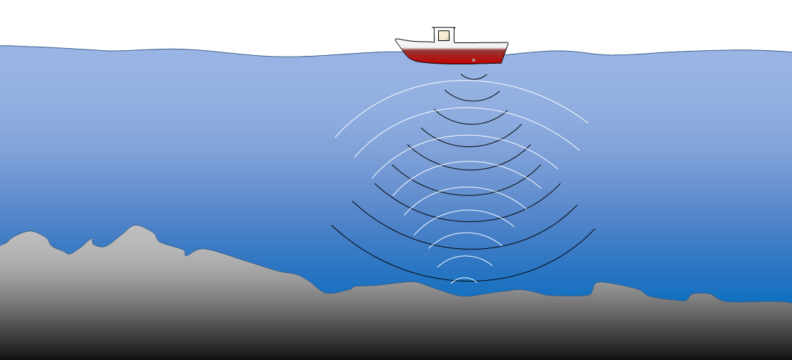
The voyage of the Challenger in 1872 and the laying of trans-Atlantic cables had shown that there were mountains beneath the seas, but most geologists and oceanographers still believed that the oceans were essentially vast basins with flat bottoms, filled with thousands of metres of sediments.
Following development of acoustic depth sounders (Figure 4.8) in the 1920s, the number of depth readings increased by many orders of magnitude, and by the 1930s there was no doubt that major mountain chains ran through all of the world’s oceans. During and after World War II, there was a well-organized campaign to study the oceans, and by 1959, sufficient bathymetric data had been collected to produce detailed maps of all the oceans (Figure 4.9).
![igure 4.9 Ocean floor bathymetry (and continental topography). Inset (a): the mid-Atlantic ridge, (b): the Newfoundland continental shelf, (c): the Nazca trench adjacent to South America, and (d): the Hawaiian Island chain. [SE after NOAA, http://bit.ly/1OtRMc0]](https://openpress.usask.ca/app/uploads/sites/29/2017/05/bathymetry.png "Chapter 1. Introduction to Geology")
- Extensive linear ridges (commonly in the central parts of the oceans) with water depths in the order of 2,000 to 3,000 m (Figure 4.9, inset a)
- Fracture zones perpendicular to the ridges (inset a)
- Deep-ocean plains at depths of 5,000 to 6,000 m (insets a and d)
- Relatively flat and shallow continental shelves with depths under 500 m (inset b)
- Deep trenches (up to 11,000 m deep), most near the continents (inset c)
- Seamounts and chains of seamounts (inset d)
Seismic Reflection Sounding
Seismic reflection sounding involves transmitting high-energy sound bursts and then measuring the echoes with a series of geophones towed behind a ship. The technique is related to acoustic sounding as described above, however, much more energy is transmitted and the sophistication of the data processing is much greater. As the technique evolved, and the amount of energy was increased, it became possible to see through the sea-floor sediments and map the bedrock topography and crustal thickness. Hence sediment thicknesses could be mapped (Figure 4.10).
![Figure 4.10 Map of global sediment thickness. [Source: NOAA, http://1.usa.gov/1Ywxxz6]](https://openpress.usask.ca/app/uploads/sites/29/2017/05/sedthick9.jpg "Chapter 1. Introduction to Geology")

With developments of networks of seismographic stations in the 1950s, it became possible to plot the locations and depths of both major and minor earthquakes with great accuracy. It was found that there is a remarkable correspondence between earthquakes and both the mid-ocean ridges and the deep ocean trenches. In 1954 Gutenberg and Richter showed that the ocean-ridge earthquakes were all relatively shallow, and confirmed what had first been shown by Benioff in the 1930s — that earthquakes in the vicinity of ocean trenches were both shallow and deep, but that the deeper ones were situated progressively farther inland from the trenches (Figure 4.12).
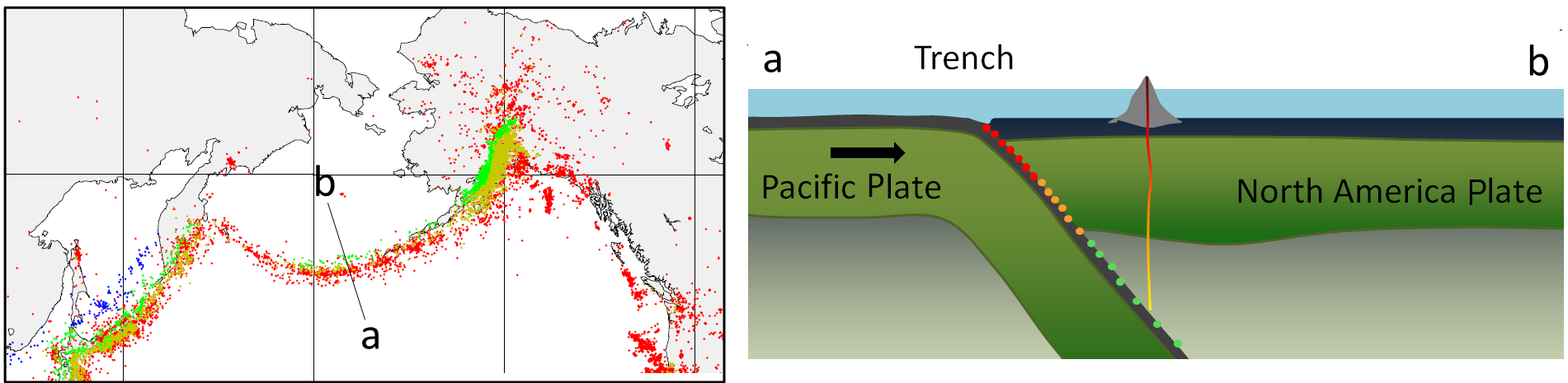
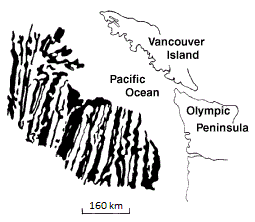
Hess proposed that new sea floor was generated from mantle material at the ocean ridges, and that old sea floor was dragged down at the ocean trenches and re-incorporated into the mantle. He suggested that the process was driven by mantle convection currents, rising at the ridges and descending at the trenches (Figure 4.14). He also suggested that the less-dense continental crust did not descend with oceanic crust into trenches, but that colliding land masses were thrust up to form mountains.
Hess’s theory formed the basis for our ideas on sea-floor spreading and continental drift, but it did not deal with the concept that the crust is made up of specific plates. Although the Hess model was not roundly criticized, it was not widely accepted (especially in the U.S.), partly because it was not well supported by hard evidence.
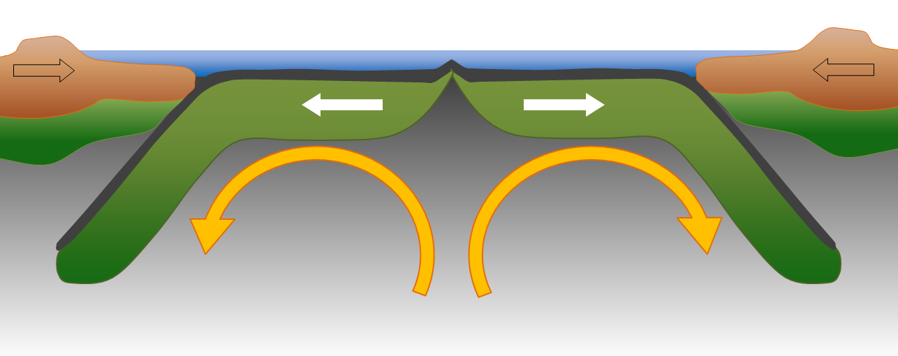
At the same time, other researchers, led by groups in California and New Zealand, were studying the phenomenon of reversals in Earth’s magnetic field. They were trying to determine when such reversals had taken place over the past several million years by analyzing the magnetic characteristics of hundreds of samples from basaltic flows. As discussed in Chapter 9, it is evident that Earth’s magnetic field becomes weakened periodically and then virtually non-existent, before becoming re-established with the reverse polarity. During periods of reversed polarity, a compass would point south instead of north.
The time scale of magnetic reversals is irregular. For example, the present “normal” event, known as the Bruhnes magnetic chron, has persisted for about 780,000 years. This was preceded by a 190,000-year reversed event; a 50,000-year normal event known as Jaramillo; and then a 700,000-year reversed event (see Figure 3.15).
In a paper published in September 1963, Vine and his PhD supervisor Drummond Matthews proposed that the patterns associated with ridges were related to the magnetic reversals, and that oceanic crust created from cooling basalt during a normal event would have polarity aligned with the present magnetic field, and thus would produce a positive anomaly (a black stripe on the sea-floor magnetic map), whereas oceanic crust created during a reversed event would have polarity opposite to the present field and thus would produce a negative magnetic anomaly (a white stripe). The same idea had been put forward a few months earlier by Lawrence Morley, of the Geological Survey of Canada; however, his papers submitted earlier in 1963 to Nature and The Journal of Geophysical Research were rejected. Many people refer to the idea as the Vine-Matthews-Morley (VMM) hypothesis.
Vine, Matthews, and Morley were the first to show this type of correspondence between the relative widths of the stripes and the periods of the magnetic reversals. The VMM hypothesis was confirmed within a few years when magnetic data were compiled from spreading ridges around the world. It was shown that the same general magnetic patterns were present straddling each ridge, although the widths of the anomalies varied according to the spreading rates characteristic of the different ridges. It was also shown that the patterns corresponded with the chronology of Earth’s magnetic field reversals. This global consistency provided strong support for the VMM hypothesis and led to rejection of the other explanations for the magnetic anomalies.
In 1963, J. Tuzo Wilson of the University of Toronto proposed the idea of a mantle plume or hot spot — a place where hot mantle material rises in a stationary and semi-permanent plume, and affects the overlying crust. He based this hypothesis partly on the distribution of the Hawaiian and Emperor Seamount island chains in the Pacific Ocean (Figure 4.15). The volcanic rock making up these islands gets progressively younger toward the southeast, culminating with the island of Hawaii itself, which consists of rock that is almost all younger than 1 Ma.
![Figure 4.15 The ages of the Hawaiian Islands and the Emperor Seamounts in relation to the location of the Hawaiian mantle plume [SE. Basemap from the National Geophysical Data Centre, accessed at: http://en.wikipedia.org/wiki/Hotspot_(geology)#/ media/File:Hawaii_hotspot.jpg.]](https://openpress.usask.ca/app/uploads/sites/29/2017/05/image0312.png "Chapter 1. Introduction to Geology")
Exercise 4.2 Volcanoes and the rate of plate motion
The Hawaiian and Emperor volcanoes shown in Figure 4.15 are listed in the table below along with their ages and their distances from the centre of the mantle plume under Hawaii (the Big Island).
| Age (Ma) | Distance (km) | Rate (cm/y) | |
| Hawaii | 0 | 0 | – |
| Necker | 10.3 | 1,058 | 10.2 |
| Midway | 27.7 | 2,432 | |
| Koko | 48.1 | 3,758 | |
| Suiko | 64.7 | 4,860 |
Plot the data on the graph provided here, and use the numbers in the table to estimate the rates of plate motion for the Pacific Plate in cm/year. (The first two are plotted for you.)
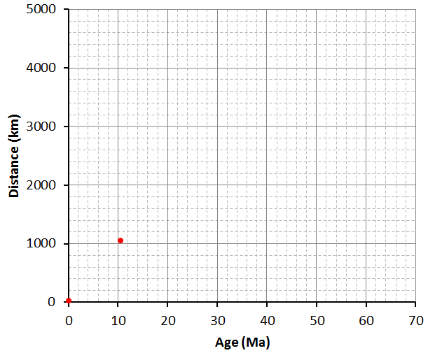
There is evidence of many such mantle plumes around the world (Figure 4.16). Most are within the ocean basins — including places like Hawaii, Iceland, and the Galapagos Islands — but some are under continents. One example is the Yellowstone hot spot in the west-central United States, and another is the one responsible for the Anahim Volcanic Belt in central British Columbia. It is evident that mantle plumes are very long-lived phenomena, lasting for at least tens of millions of years, possibly for hundreds of millions of years in some cases.
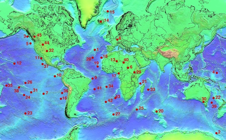
Although oceanic spreading ridges appear to be curved features on Earth’s surface, in fact the ridges are composed of a series of straight-line segments, offset at intervals by faults perpendicular to the ridge (Figure 4.17). In a paper published in 1965, Tuzo Wilson termed these features transform faults. He described the nature of the motion along them, and showed why there are earthquakes only on the section of a transform fault between two adjacent ridge segments. The San Andreas Fault in California is a very long transform fault that links the southern end of the Juan de Fuca spreading ridge to the East Pacific Rise spreading ridges situated in the Gulf of California (see Figure 4.25). The Queen Charlotte Fault, which extends north from the northern end of the Juan de Fuca spreading ridge (near the northern end of Vancouver Island) toward Alaska, is also a transform fault.
![Figure 4.17 A part of the mid-Atlantic ridge near the equator. The double white lines are spreading ridges. The solid white lines are fracture zones. As shown by the yellow arrows, the relative motion of the plates on either side of the fracture zones can be similar (arrows pointing the same direction) or opposite (arrows pointing opposite directions). Transform faults (red lines) are in between the ridge segments, where the yellow arrows point in opposite directions. [SE]](https://openpress.usask.ca/app/uploads/sites/29/2017/05/image0371.png "Chapter 1. Introduction to Geology")
In the same 1965 paper, Wilson introduced the idea that the crust can be divided into a series of rigid plates, and thus he is responsible for the term plate tectonics.
Exercise 4.3 Paper transform fault model
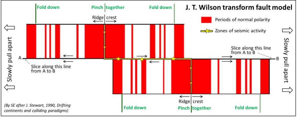
J. Tuzo Wilson used a paper model, a little bit like the one shown here, to explain transform faults to his colleagues. To use this model print this page, cut around the outside, and then slice along the line A-B (the fracture zone) with a sharp knife. Fold down the top half where shown, and then pinch together in the middle. Do the same with the bottom half. When you’re done, you should have something like the example below, with two folds of paper extending underneath. Find someone else to pinch those folds with two fingers just below each ridge crest, and then gently pull apart where shown. As you do, the oceanic crust will emerge from the middle, and you’ll see that the parts of the fracture zone between the ridge crests will be moving in opposite directions (this is the transform fault) while the parts of the fracture zone outside of the ridge crests will be moving in the same direction. You’ll also see that the oceanic crust is being magnetized as it forms at the ridge. The magnetic patterns shown are accurate, and represent the last 2.5 Ma of geological time.
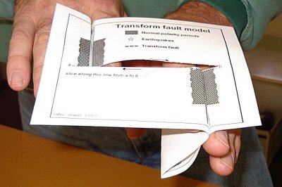
There are other versions of this model available at https://web.viu.ca/earle/transform-model/. For more information see: Earle, S., 2004, A simple paper model of a transform fault at a spreading ridge, J. Geosc. Educ. V. 52, p. 391-2.
4.4 Plates, Plate Motions, and Plate-Boundary Processes
Continental drift and sea-floor spreading became widely accepted around 1965 as more and more geologists started thinking in these terms. By the end of 1967, Earth’s surface had been mapped into a series of plates (Figure 4.18). The major plates are Eurasia, Pacific, India, Australia, North America, South America, Africa, and Antarctic. There are also numerous small plates (e.g., Juan de Fuca, Nazca, Scotia, Philippine, Caribbean), and many very small plates or sub-plates. For example the Juan de Fuca Plate is actually three separate plates (Gorda, Juan de Fuca, and Explorer) that all move in the same general direction but at slightly different rates.
![Figure 4.18 A detailed map of Earth's tectonic plates. [Source: NASA, http://bit.ly/1PZHRMZ]](https://openpress.usask.ca/app/uploads/sites/29/2017/05/Plate_tectonics_map.gif "Chapter 1. Introduction to Geology")
Plates move as rigid bodies, so it may seem surprising that the North American Plate can be moving at different rates in different places. The explanation is that plates move in a rotational manner. The North American Plate, for example, rotates counter-clockwise; the Eurasian Plate rotates clockwise.
Boundaries between the plates are of three types: divergent (i.e., moving apart), convergent (i.e., moving together), and transform (moving side by side). Before we talk about processes at plate boundaries, it’s important to point out that there are never gaps between plates. The plates are made up of crust and the lithospheric part of the mantle (Figure 4.19), and even though they are moving all the time, and in different directions, there is never a significant amount of space between them. Plates are thought to move along the lithosphere-asthenosphere boundary, as the asthenosphere is the zone of partial melting. It is assumed that the relative lack of strength of the partial melting zone facilitates the sliding of the lithospheric plates.
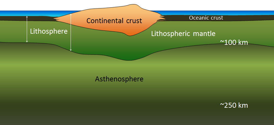
At spreading centres, the lithospheric mantle may be very thin because the upward convective motion of hot mantle material generates temperatures that are too high for the existence of a significant thickness of rigid lithosphere (Figure 4.14). The fact that the plates include both crustal material and lithospheric mantle material makes it possible for a single plate to be made up of both oceanic and continental crust. For example, the North American Plate includes most of North America, plus half of the northern Atlantic Ocean. Similarly the South American Plate extends across the western part of the southern Atlantic Ocean, while the European and African plates each include part of the eastern Atlantic Ocean. The Pacific Plate is almost entirely oceanic, but it does include the part of California west of the San Andreas Fault.
Divergent Boundaries
Divergent boundaries are spreading boundaries, where new oceanic crust is created from magma derived from partial melting of the mantle caused by decompression as hot mantle rock from depth is moved toward the surface (Figure 4.20, bottom left).
The triangular zone of partial melting near the ridge crest is approximately 60 km thick and the proportion of magma is about 10% of the rock volume, thus producing crust that is about 6 km thick. Most divergent boundaries are located at the oceanic ridges (although some are on land), and the crustal material created at a spreading boundary is always oceanic in character; in other words, it is mafic igneous rock (e.g., basalt or gabbro, with minerals rich in iron and magnesium). Spreading rates vary considerably, from 1 cm/y to 3 cm/y in the Atlantic, to between 6 cm/y and 10 cm/y in the Pacific. Some of the processes taking place in this setting include (Figure 4.20, top):
- Magma from the mantle pushing up to fill the voids left by divergence of the two plates
- Pillow lavas forming where magma is pushed out into seawater (Figure 4.20, bottom right)
- Vertical sheeted dykes intruding into cracks resulting from the spreading
- Magma cooling more slowly in the lower part of the new crust and forming gabbro bodies
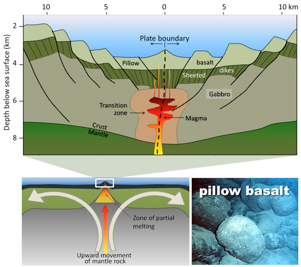
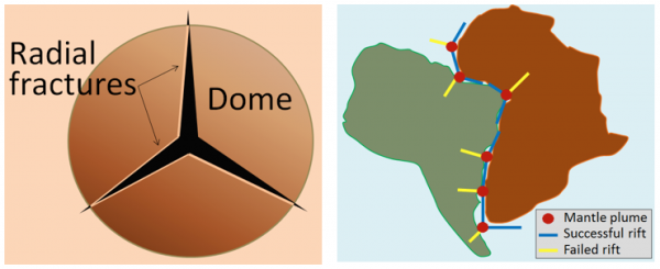
When a series of mantle plumes exists beneath a large continent, the resulting rifts may align and lead to the formation of a rift valley (such as the present-day Great Rift Valley in eastern Africa). It is suggested that this type of valley eventually develops into a linear sea (such as the present-day Red Sea), and finally into an ocean (such as the Atlantic). It is likely that as many as 20 mantle plumes, many of which still exist, were responsible for the initiation of the rifting of Pangea along what is now the mid-Atlantic ridge (see Figure 4.16).
Convergent Boundaries
Convergent boundaries, where two plates are moving toward each other, are of three types, depending on whether ocean or continental crust is present on either side of the boundary. The types are ocean-ocean, ocean-continent, and continent-continent.
Ocean-Ocean Convergent Boundaries
At an ocean-ocean convergent boundary (Figure 4.22), one of the plates (oceanic crust and lithospheric mantle) is pushed, or subducted, under the other. Often it is the older and colder plate that is denser and subducts beneath the younger and hotter plate. There is commonly an ocean trench along the boundary. The subducted lithosphere descends into the hot mantle at a relatively shallow angle close to the subduction zone, but at steeper angles farther down (up to about 45°).
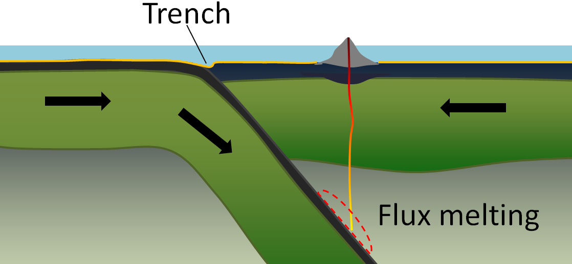
The newly produced magma, which is lighter than the surrounding mantle material, rises through the mantle and the overlying oceanic crust to the ocean floor where it creates a chain of volcanic islands known as an island arc. A mature island arc develops into a chain of relatively large islands (such as Japan or Indonesia) as more and more volcanic material is extruded and sedimentary rocks accumulate around the islands.
As described above in the context of Benioff zones (Figure 4.12), earthquakes take place close to the boundary between the subducting crust and the overriding crust. The largest earthquakes occur near the surface where the subducting plate is still cold and strong.
Examples of ocean-ocean convergent zones are subduction of the Pacific Plate south of Alaska (Aleutian Islands) and west of the Philippines, subduction of the India Plate south of Indonesia, and subduction of the Atlantic Plate beneath the Caribbean Plate.
Ocean-Continent Convergent Boundaries
At an ocean-continent convergent boundary, the oceanic plate is pushed under the continental plate in the same manner as at an ocean-ocean boundary. Sediment that has accumulated on the continental slope is thrust up into an accretionary wedge, and compression leads to thrusting within the continental plate (Figure 4.23). The mafic magma produced adjacent to the subduction zone rises to the base of the continental crust and leads to partial melting of the crustal rock. The resulting magma ascends through the crust, producing a mountain chain with many volcanoes.
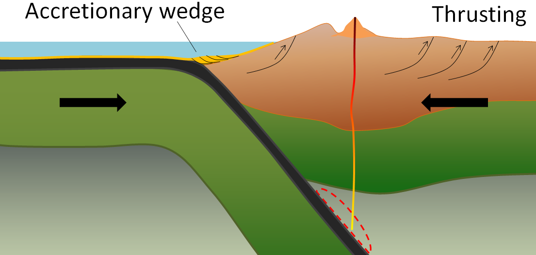
Continent-Continent Convergent Boundary
A continent-continent collision occurs when a continent or large island that has been moved along with subducting oceanic crust collides with another continent (Figure 4.24). The colliding continental material will not be subducted because it is not dense enough, but the root of the oceanic plate will eventually break off and sink into the mantle. There is tremendous deformation of the pre-existing continental rocks, and creation of mountains from that rock, from any sediments that had accumulated along the shores (i.e., within geosynclines) of both continental masses, and commonly also from some ocean crust and upper mantle material.
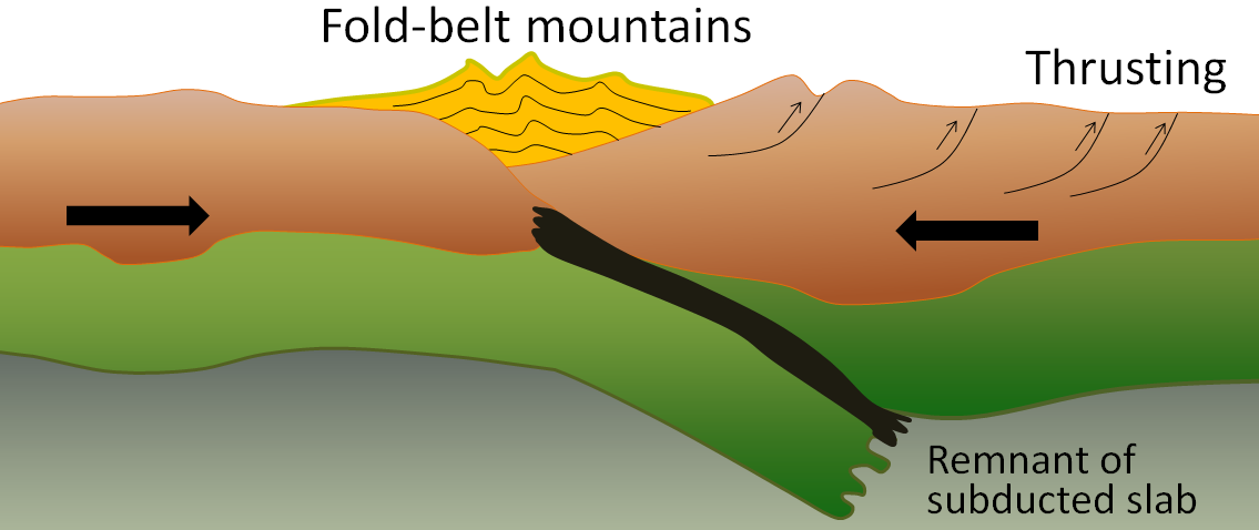
Transform Boundaries
Transform boundaries exist where one plate slides past another without producing or destroying crust.[footnote]The exception is cases where the transform boundary has bends and jogs. There will be collisions and divergence on a small scale as the jogs crash into the bends.[/footnote] As explained above, most transform faults connect segments of mid-ocean ridges and are thus ocean-ocean plate boundaries (Figure 4.17). Some transform faults connect continental parts of plates. An example is the San Andreas Fault, which connects the southern end of the Juan de Fuca Ridge with the northern end of the East Pacific Rise (ridge) in the Gulf of California (Figures 4.25 and 4.26). The part of California west of the San Andreas Fault and all of Baja California are on the Pacific Plate. Transform faults do not just connect divergent boundaries. For example, the Queen Charlotte Fault connects the north end of the Juan de Fuca Ridge, starting at the north end of Vancouver Island, to the Aleutian subduction zone.
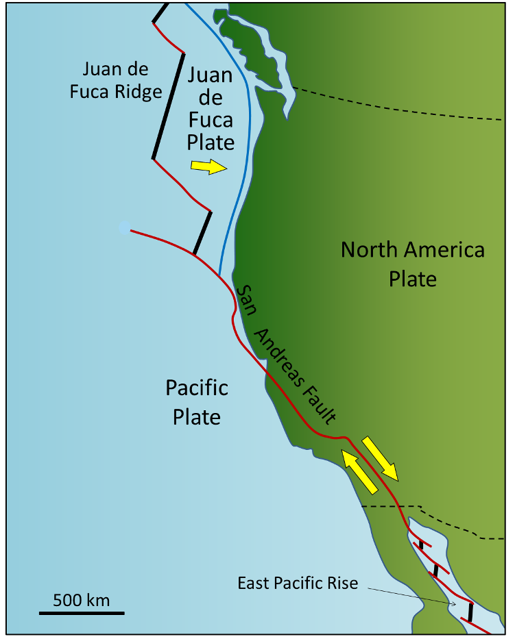
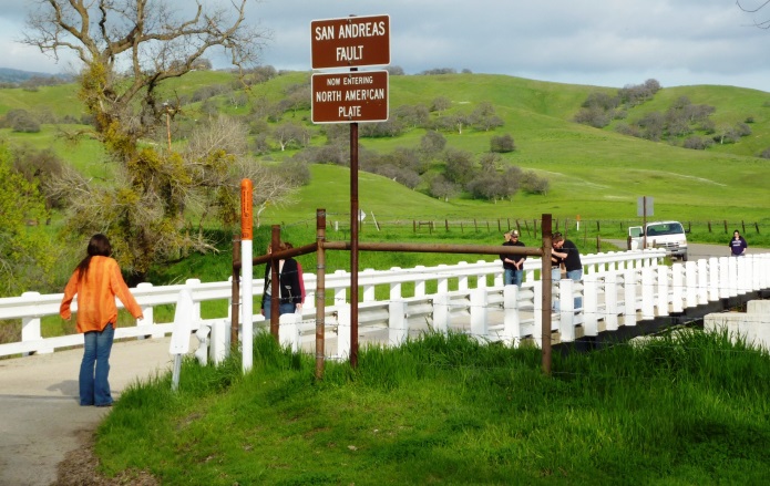
Exercise 4.4 A different type of transform fault
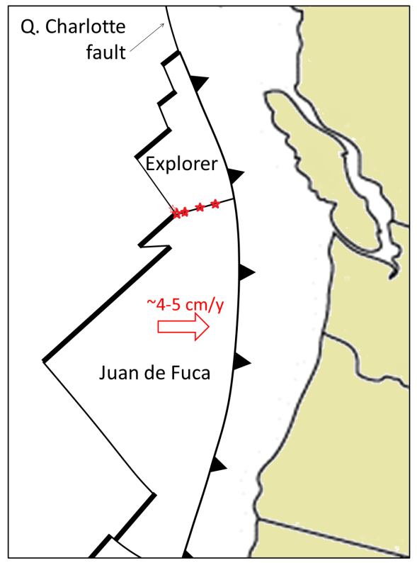
This map shows the Juan de Fuca (JDF) and Explorer Plates off the coast of Vancouver Island. We know that the JDF Plate is moving toward the North American Plate at around 4 cm/y to 5 cm/y. We think that the Explorer Plate is also moving east, but we don’t know the rate, and there is evidence that it is slower than the JDF Plate.
The boundary between the two plates is the Nootka Fault, which is the location of frequent small-to-medium earthquakes (up to magnitude ~5), as depicted by the red stars. Explain why the Nootka Fault is a transform fault, and show the relative sense of motion along the fault with two small arrows.
Plate Tectonics and Supercontinent Cycles
As originally described by Wegener in 1915, the present continents were once all part of a supercontinent, which he termed Pangea (all land). More recent studies of continental matchups and the magnetic ages of ocean-floor rocks have enabled us to reconstruct the history of the break-up of Pangea.
Pangea began to rift apart along a line between Africa and Asia and between North America and South America at around 200 Ma (Figure 4.27). During the same period the Atlantic Ocean began to open up between northern Africa and North America, and India broke away from Antarctica. Between 200 and 150 Ma, rifting started between South America and Africa and between North America and Europe, and India moved north toward Asia. By 80 Ma, Africa had separated from South America, most of Europe had separated from North America, and India had separated from Antarctica. By 50 Ma, Australia had separated from Antarctic, and shortly after that, India collided with Asia.
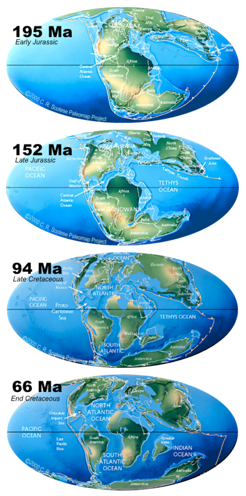
Pangea was not the first supercontinent. It was preceded by Pannotia (600 to 540 Ma), Rodinia (1,100 to 750 Ma), and by others before that. In fact, in 1966, Tuzo Wilson proposed that supercontinents are part of an on-going cycle, which we now refer to as a Wilson cycle. In a Wilson cycle, supercontinents break up, and fragments drift apart only to collide again and make a new supercontinent.
At present we are in the stages of a Wilson cycle where fragments are drifting and changing their configuration. North and South America, Europe, and Africa are moving with their respective portions of the Atlantic Ocean. The eastern margins of North and South America and the western margins of Europe and Africa are called passive margins because there is no subduction taking place along them. Because the oceanic crust formed by spreading on the mid-Atlantic ridge is not currently being subducted (except in the Caribbean), the Atlantic Ocean is slowly getting bigger, and the Pacific Ocean is getting smaller.
This situation may not continue for too much longer, however. As the Atlantic Ocean floor gets weighed down around its margins by great thickness of continental sediments (i.e., geosynclines), it will be pushed farther and farther into the mantle, and eventually the oceanic lithosphere may break away from the continental lithosphere (Figure 4.28).
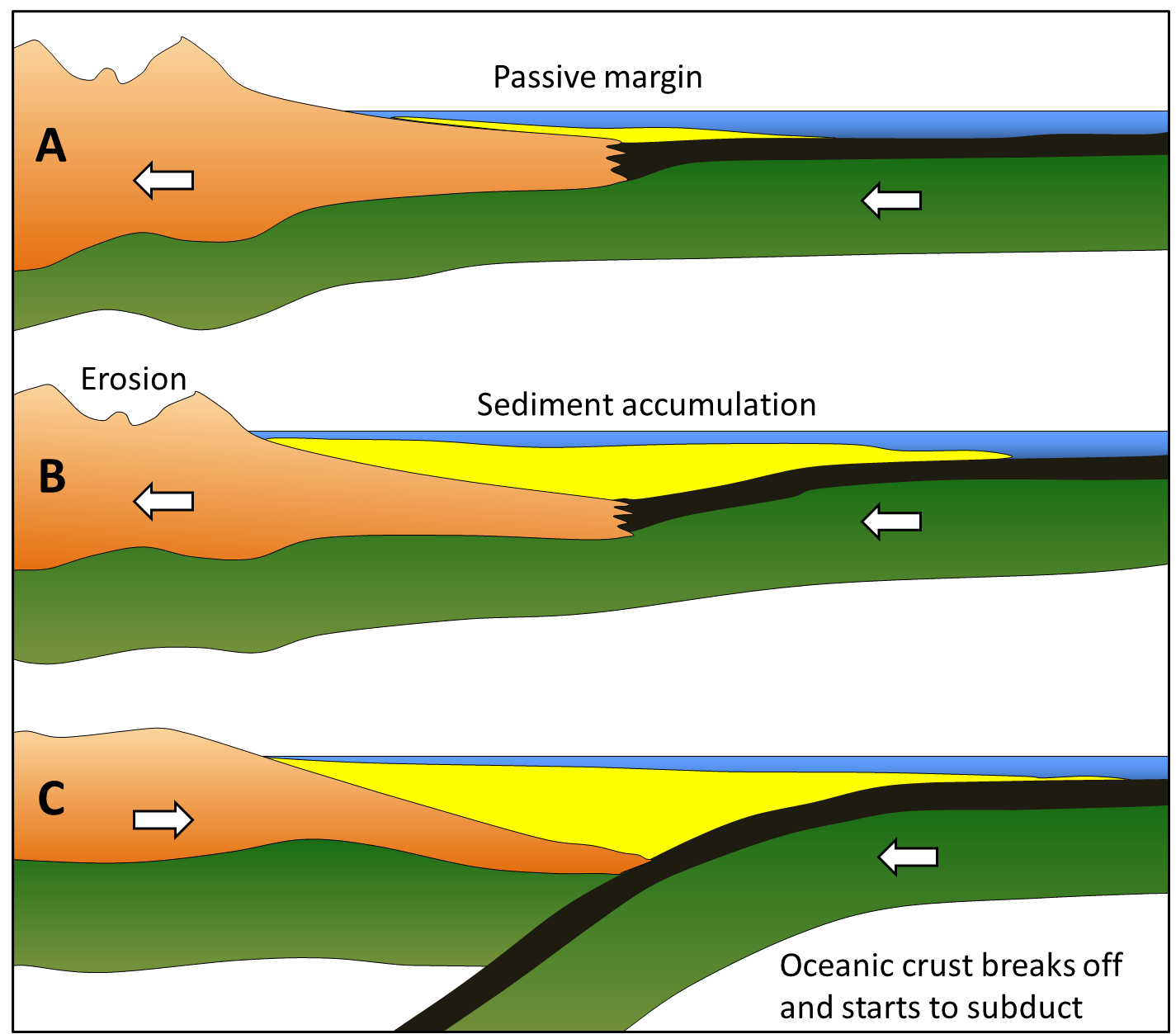
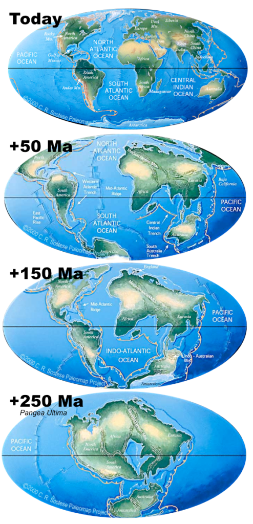
The apparent line of collision runs between Norway and Sweden, between Scotland and England, through Ireland, through Newfoundland, and the Maritimes, through the northeastern and eastern states, and across the northern end of Florida. When rifting of Pangea started at approximately 200 Ma, the fissuring was along a different line from the line of the earlier collision. This is why some of the mountain chains formed during the earlier collision can be traced from Europe to North America and from Europe to Africa.
It is probably no coincidence that the Atlantic Ocean rift may have occurred in approximately the same place during two separate events several hundred million years apart. The series of hot spots that has been identified in the Atlantic Ocean may also have existed for several hundred million years, and thus may have contributed to rifting in roughly the same place on at least two separate occasions (Figure 4.30).
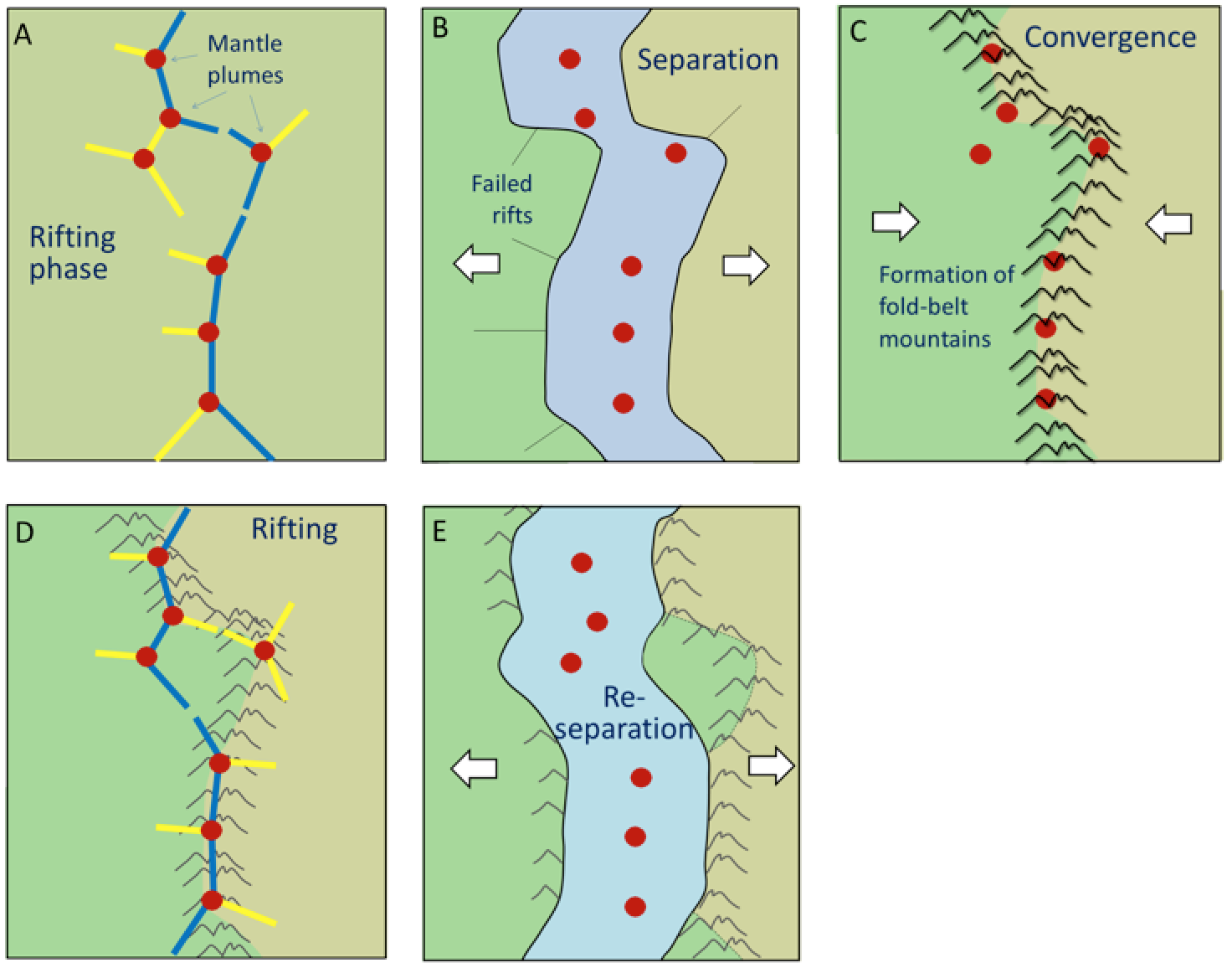
4.5 Mechanisms for Plate Motion
Mantle convection is often said to be critical to plate tectonics. While this is almost certainly so, there is still debate about the actual forces that make the plates move. One side of the argument holds that the plates are only moved by the traction caused by mantle convection- that friction between the asthenosphere and lithosphere pulls the lithosphere along as the mantle convects. The other side holds that traction plays only a minor role and that ridge-push and slab-pull are more important (Figure 4.31).
Ridge-push refers to gravity causing lithosphere to slide downhill away from where convection is pushing mid-ocean ridges upward. Slab-pull refers to the weight of subducting slabs dragging the rest of the plate down into the mantle.

- Plates that are attached to subducting slabs (e.g., Pacific, Australian, and Nazca Plates) move the fastest, and plates that are not (e.g., North American, South American, Eurasian, and African Plates) move significantly slower.
- In order for the traction model to apply, the mantle would have to be moving about five times faster than the plates are moving (because the coupling between the partially liquid asthenosphere and the plates is not strong), and such high rates of convection are not supported by geophysical models.
- Although large plates have potential for much higher convection traction, plate velocity is not related to plate area.
Although ridge-push/slab-pull is the favoured mechanism for plate motion, it’s important not to underestimate the role of mantle convection. Without convection, there would be no ridges to push from because upward convection brings hot buoyant rock to surface. Furthermore, many plates, including our own North American Plate, move along nicely — albeit slowly — without any slab-pull happening.
Chapter 4 Summary
The topics covered in this chapter can be summarized as follows:
4.1 Alfred Wegener – The Father of Plate Tectonics
The evidence for continental drift in the early 20th century included the matching of continental shapes on either side of the Atlantic and the geological and fossil matchups between continents that are now thousands of kilometres apart.
4.2 Global Geological Models of the Early 20th Century
The established theories of global geology were permanentism and contractionism, but neither of these theories was able to explain some of the evidence that supported the idea of continental drift.
4.3 Geological Renaissance of the Mid-20th Century
Giant strides were made in understanding Earth during the middle decades of the 20th century, including discovering magnetic evidence of continental drift, mapping the topography of the ocean floor, describing the depth relationships of earthquakes along ocean trenches, measuring heat flow differences in various parts of the ocean floor, and mapping magnetic reversals on the sea floor. By the mid-1960s, the fundamentals of the theory of plate tectonics were in place.
4.4 Plates, Plate Motions, and Plate-Boundary Processes
Earth’s lithosphere is made up of over 20 plates that are moving in different directions at rates of between 1 cm/y and 10 cm/y. The three types of plate boundaries are divergent (plates moving apart and new crust forming), convergent (plates moving together and one being subducted), and transform (plates moving side by side). Divergent boundaries form where existing plates are rifted apart, and it is hypothesized that this is caused by a series of mantle plumes. Subduction zones are assumed to form where accumulation of sediment at a passive margin leads to separation of oceanic and continental lithosphere. Supercontinents form and break up through these processes.
4.5 Mechanisms for Plate Motion
It is widely believed that ridge-push and slab-pull are the main mechanisms for plate motion, as opposed to traction by mantle convection. Mantle convection is a key factor for producing the conditions necessary for ridge-push and slab-pull.
Questions for Review
- List some of the evidence used by Wegener to support his idea of moving continents.
- What was the primary technical weakness with Wegener’s continental drift theory?
- How were mountains thought to be formed (a) by contractionists and (b) by permanentists?
- How were the trans-Atlantic paleontological matchups explained in the late 19th century?
- In the context of isostasy, what would prevent an area of continental crust from becoming part of an ocean?
- How did we learn about the topography of the sea floor in the early part of the 20th century?
- How does the temperature profile of the crust and the mantle indicate that part of the mantle must be convecting?
- What evidence from paleomagnetic studies provided support for continental drift?
- Which parts of the oceans are the deepest?
- Why is there less sediment in the ocean ridge areas than in other parts of the sea floor?
- How were the oceanic heat-flow data related to mantle convection?
- Describe the spatial and depth distribution of earthquakes at ocean ridges and ocean trenches.
- In the model for ocean basins developed by Harold Hess, what took place at oceanic ridges and what took place at oceanic trenches?
- What aspect of plate tectonics was not included in the Hess theory?
- What is a mantle plume and what is its expected lifespan?
- Describe the nature of movement at an ocean ridge transform fault (a) between the ridge segments, and (b) outside the ridge segments.
- How is it possible for a plate to include both oceanic and continental crust?
- What is the likely relationship between mantle plumes and the development of a continental rift?
- Why does subduction not take place at a continent-continent convergent zone?
- Where are Earth’s most recent sites of continental rifting and creation of new ocean floor?
- What is likely to happen to western California over the next 50 million years?
- What geological situation might eventually lead to the generation of a subduction zone at a passive ocean-continent boundary such as the eastern coast of North America?
19.1 The Geological Time Scale
William “Strata” Smith worked as a surveyor in the coal-mining and canal-building industries in southwestern England in the late 1700s and early 1800s. While doing his work, he had many opportunities to look at the Paleozoic and Mesozoic sedimentary rocks of the region, and he did so in a way that few had done before. Smith noticed the textural similarities and differences between rocks in different locations, and more importantly, he discovered that fossils could be used to correlate rocks of the same age. Smith is credited with formulating the principle of faunal succession (the concept that specific types of organisms lived during different time intervals), and he used it to great effect in his monumental project to create a geological map of England and Wales, published in 1815. (For more on William Smith, including a large-scale digital copy of the famous map, see http://en.wikipedia.org/wiki/William_Smith_%28geologist%29.)
Inset into Smith’s great geological map is a small diagram showing a schematic geological cross-section extending from the Thames estuary of eastern England all the way to the west coast of Wales. Smith shows the sequence of rocks, from the Paleozoic rocks of Wales and western England, through the Mesozoic rocks of central England, to the Cenozoic rocks of the area around London (Figure 19.2). Although Smith did not put any dates on these — because he didn’t know them — he was aware of the principle of superposition (the idea, developed much earlier by the Danish theologian and scientist Nicholas Steno, that young sedimentary rocks form on top of older ones), and so he knew that this diagram represented a stratigraphic column. And because almost every period of the Phanerozoic is represented along that section through Wales and England, it is a primitive geological time scale.
![Figure 8.2 William Smith’s “Sketch of the succession of strata and their relative altitudes,” an inset on his geological map of England and Wales (with era names added). [SE after: http://earthobservatory.nasa.gov/Features/WilliamSmith/images/sketch_of_the_succession_of_strata.jpg]](https://openpress.usask.ca/app/uploads/sites/29/2017/05/geological-map-of-England-and-Wales-e1439316487427.png "Chapter 1. Introduction to Geology")
The early time scales were only relative because 19th century geologists did not know the ages of the rocks. That information was not available until the development of isotopic dating techniques early in the 20th century.
The geological time scale is currently maintained by the International Commission on Stratigraphy (ICS), which is part of the International Union of Geological Sciences. The time scale is continuously being updated as we learn more about the timing and nature of past geological events. You can view the ICS time scale at http://www.stratigraphy.org/index.php/ics-chart-timescale. It would be a good idea to print a copy (in colour) to put on your wall while you are studying geology.
Geological time has been divided into four eons: Hadean, Archean, Proterozoic, and Phanerozoic, and as shown in Figure 19.3, the first three of these represent almost 90% of Earth’s history. The last one, the Phanerozoic (meaning “visible life”), is the time that we are most familiar with because Phanerozoic rocks are the most common on Earth, and they contain evidence of the life forms that we are all somewhat familiar with.

![Figure 8.4 The eras (middle row) and periods (bottom row) of the Phanerozoic [SE]](https://openpress.usask.ca/app/uploads/sites/29/2017/05/Phanerozoic.png "Chapter 1. Introduction to Geology")
![Figure 8.5 The periods (middle row) and epochs (bottom row) of the Cenozoic [SE]](https://openpress.usask.ca/app/uploads/sites/29/2017/05/Cenozoic.png "Chapter 1. Introduction to Geology")
19.2 Relative Dating Methods
The simplest and most intuitive way of dating geological features is to look at the relationships between them. There are a few simple rules for doing this. For example, the principle of superposition states that sedimentary layers are deposited in sequence, and, unless the entire sequence has been turned over by tectonic processes or disrupted by faulting, the layers at the bottom are older than those at the top. The principle of inclusions states that any rock fragments that are included in rock must be older than the rock in which they are included. For example, a xenolith in an igneous rock or a clast in sedimentary rock must be older than the rock that includes it (Figure 19.6).
![Figure 8.6a A xenolith of diorite incorporated into a basalt lava flow, Mauna Kea volcano, Hawaii. The lava flow took place some time after the diorite cooled, was uplifted, and then eroded. (Hammerhead for scale) [SE]](https://openpress.usask.ca/app/uploads/sites/29/2017/05/xenolith-of-diorite.jpg "Chapter 1. Introduction to Geology")
![Figure 8.6b Rip-up clasts of shale embedded in Gabriola Formation sandstone, Gabriola Island, B.C. The pieces of shale were eroded as the sandstone was deposited, so the shale is older than the sandstone. [SE]](https://openpress.usask.ca/app/uploads/sites/29/2017/05/sandstone.jpg "Chapter 1. Introduction to Geology")
The principle of cross-cutting relationships states that any geological feature that cuts across, or disrupts another feature must be younger than the feature that is disrupted. An example of this is given in Figure 19.7, which shows three different sedimentary layers. The lower sandstone layer is disrupted by two faults, so we can infer that the faults are younger than that layer. But the faults do not appear to continue into the coal seam, and they certainly do not continue into the upper sandstone. So we can infer that coal seam is younger than the faults (because it disrupts them), and of course the upper sandstone is youngest of all, because it lies on top of the coal seam.
![Figure 8.7 Superposition and cross-cutting relationships in Cretaceous Nanaimo Group rocks in Nanaimo, B.C. The coal seam is about 50 cm thick. [SE ]](https://openpress.usask.ca/app/uploads/sites/29/2017/05/Cretaceous-Nanaimo.png "Chapter 1. Introduction to Geology")
Exercise 19.1 Cross-Cutting Relationships
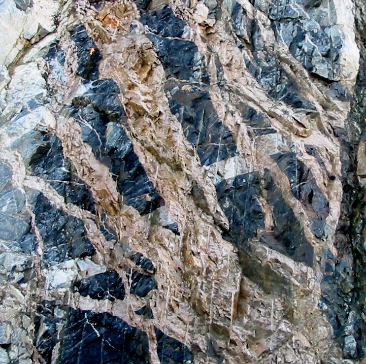
The outcrop shown here (from Horseshoe Bay, B.C.) has three main rock types:
1. Buff/pink felsic intrusive igneous rock present as somewhat irregular masses trending from lower right to upper left
2. Dark grey metamorphosed basalt
3. A 50 cm wide light-grey felsic intrusive igneous dyke extending from the lower left to the middle right – offset in several places
Using the principle of cross-cutting relationships outlined above, determine the relative ages of these three rock types.
(The near-vertical stripes are blasting drill holes. The image is about 7 m across.)
An unconformity represents an interruption in the process of deposition of sedimentary rocks. Recognizing unconformities is important for understanding time relationships in sedimentary sequences. An example of an unconformity is shown in Figure 19.8. The Proterozoic rocks of the Grand Canyon Group have been tilted and then eroded to a flat surface prior to deposition of the younger Paleozoic rocks. The difference in time between the youngest of the Proterozoic rocks and the oldest of the Paleozoic rocks is close to 300 million years. Tilting and erosion of the older rocks took place during this time, and if there was any deposition going on in this area, the evidence of it is now gone.
![Figure 8.8 The great angular unconformity in the Grand Canyon, Arizona. The tilted rocks at the bottom are part of the Proterozoic Grand Canyon Group (aged 825 to 1,250 Ma). The flat-lying rocks at the top are Paleozoic (540 to 250 Ma). The boundary between the two (which is marked, where visible, with a dashed white line) represents a time gap of nearly 300 million years. [SE ]](https://openpress.usask.ca/app/uploads/sites/29/2017/05/Grand-Canyon.jpg "Chapter 1. Introduction to Geology")
| Unconformity Type | Description |
| Nonconformity | A boundary between non-sedimentary rocks (below) and sedimentary rocks (above) |
| Angular unconformity | A boundary between two sequences of sedimentary rocks where the underlying ones have been tilted (or folded) and eroded prior to the deposition of the younger ones (as in Figure 19.8) |
| Disconformity | A boundary between two sequences of sedimentary rocks where the underlying ones have been eroded (but not tilted) prior to the deposition of the younger ones (as in Figure 19.7) |
| Paraconformity | A time gap in a sequence of sedimentary rocks that does not show up as an angular unconformity or a disconformity |
Table 19.1 The characteristics of the four types of unconformities
![Figure 8.9 The four types of unconformities: a: a nonconformity between non-sedimentary rock and sedimentary rock, b: an angular unconformity , c: a disconformity between layers of sedimentary rock, where the older rock has been eroded but not tilted, and d: a paraconformity where there is a long period (millions of years) of non-deposition between two parallel layers. [SE ]](https://openpress.usask.ca/app/uploads/sites/29/2017/05/unconformities.png "Chapter 1. Introduction to Geology")
19.3 Dating Rocks Using Fossils
Geologists get a wide range of information from fossils. They help us to understand evolution and life in general; they provide critical information for understanding depositional environments and changes in Earth’s climate; and, of course, they can be used to date rocks.
Although the recognition of fossils goes back hundreds of years, the systematic cataloguing and assignment of relative ages to different organisms from the distant past — paleontology — only dates back to the earliest part of the 19th century. The oldest undisputed fossils are from rocks dated around 3.5 Ga, and although fossils this old are typically poorly preserved and are not useful for dating rocks, they can still provide important information about conditions at the time. The oldest well-understood fossils are from rocks dating back to around 600 Ma, and the sedimentary record from that time forward is rich in fossil remains that provide a detailed record of the history of life. However, as anyone who has gone hunting for fossils knows, that does not mean that all sedimentary rocks have visible fossils or that they are easy to find. Fossils alone cannot provide us with numerical ages of rocks, but over the past century geologists have acquired enough isotopic dates from rocks associated with fossil-bearing rocks (such as igneous dykes cutting through sedimentary layers) to be able to put specific time limits on most fossils.
A very selective history of life on Earth over the past 600 million years is provided in Figure 19.10. The major groups of organisms that we are familiar with evolved between the late Proterozoic and the Cambrian (~600 Ma to ~520 Ma). Plants, which evolved in the oceans as green algae, came onto land during the Ordovician (~450 Ma). Insects, which evolved from marine arthropods, came onto land during the Devonian (400 Ma), and amphibians (i.e., vertebrates) came onto land about 50 million years later. By the late Carboniferous, trees had evolved from earlier plants, and reptiles had evolved from amphibians. By the mid-Triassic, dinosaurs and mammals had evolved from very different branches of the reptiles; birds evolved from dinosaurs during the Jurassic. Flowering plants evolved in the late Jurassic or early Cretaceous. The earliest primates evolved from other mammals in the early Paleogene, and the genus Homo evolved during the late Neogene (~2.8 Ma).
![Figure 8.10 A summary of life on Earth during the late Proterozoic and the Phanerozoic. The top row shows geological eras, and the lower row shows the periods. [SE]](https://openpress.usask.ca/app/uploads/sites/29/2017/05/Proterozoic-and-the-Phanerozoic.png "Chapter 1. Introduction to Geology")
The Phanerozoic has seen five major extinctions, as indicated in Figure 19.10. The most significant of these was at the end of the Permian, which saw the extinction of over 80% of all species and over 90% of all marine species. Most well-known types of organisms were decimated by this event, but only a few became completely extinct, including trilobites. The second most significant extinction was at the Cretaceous-Paleogene boundary (K-Pg, a.k.a. the K-T extinction). At that time, about 75% of marine species disappeared. Again, a few well-known types of organisms disappeared altogether, including dinosaurs (but not birds) and the pterosaurs. Other types were badly decimated but survived, and then flourished in the Paleogene. The K-Pg extinction is thought to have been caused by the impact of a large extraterrestrial body (10 km to 15 km across), but it is generally agreed that the other four Phanerozoic extinctions had other causes, although their exact nature is not clearly understood.
As already stated, it is no coincidence that the major extinctions all coincide with boundaries of geological periods and even eras. Paleontologists have placed most of the divisions of the geological time scale at points in the fossil record where there are major changes in the type of organisms observed.
If we can identify a fossil to the species level, or at least to the genus level, and we know the time period when the organism lived, we can assign a range of time to the rock. That range might be several million years because some organisms survived for a very long time. If the rock we are studying has several types of fossils in it, and we can assign time ranges to those fossils, we might be able to narrow the time range for the age of the rock considerably. An example of this is given in Figure 19.11.
![Figure 8.11 The application of bracketing to constrain the age of a rock based on several fossils. In this diagram, the coloured bar represents the time range during which each of the four species (A – D) existed on Earth. Although each species lived for several million years, we can narrow down the likely age of the rock to just 0.7 Ma during which all four species co-existed. [SE]](https://openpress.usask.ca/app/uploads/sites/29/2017/05/age-of-a-rock.png "Chapter 1. Introduction to Geology")
Some organisms survived for a very long time, and are not particularly useful for dating rocks. Sharks, for example, have been around for over 400 million years, and the great white shark has survived for 16 million years, so far. Organisms that lived for relatively short time periods are particularly useful for dating rocks, especially if they were distributed over a wide geographic area and so can be used to compare rocks from different regions. These are known as index fossils. There is no specific limit on how short the time span has to be to qualify as an index fossil. Some lived for millions of years, and others for much less than a million years.
Some well-studied groups of organisms qualify as biozone fossils because, although the genera and families lived over a long time, each species lived for a relatively short time and can be easily distinguished from others on the basis of specific features. For example, ammonites have a distinctive feature known as the suture line — where the internal shell layers that separate the individual chambers (septae) meet the outer shell wall, as shown in Figure 19.12. These suture lines are sufficiently variable to identify species that can be used to estimate the relative or absolute ages of the rocks in which they are found.
![Figure 8.12 The septum of an ammonite (white part, left), and the suture lines where the septae meet the outer shell (right). [SE]](https://openpress.usask.ca/app/uploads/sites/29/2017/05/septum-of-an-ammonite.png "Chapter 1. Introduction to Geology")
Foraminifera (small, carbonate-shelled marine organisms that originated during the Triassic and are still around today) are also useful biozone fossils. As shown in Figure 19.13, numerous different foraminifera lived during the Cretaceous. Some lasted for over 10 million years, but others for less than 1 million years. If the foraminifera in a rock can be identified to the species level, we can get a good idea of its age.
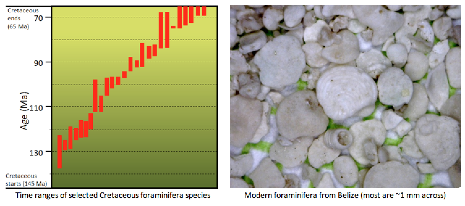
Exercise 19.2 Dating Rocks Using Index Fossils
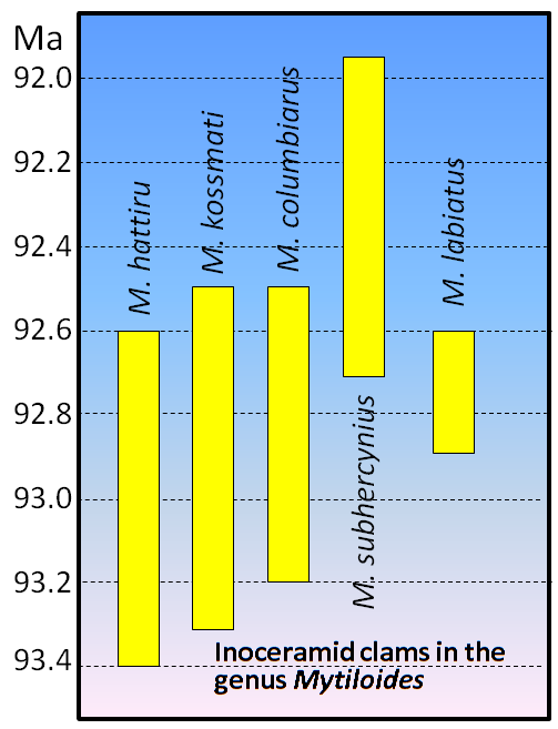
How would that change if M. subhercynius was not present in these rocks?
19.4 Isotopic Dating Methods
Originally fossils only provided us with relative ages because, although early paleontologists understood biological succession, they did not know the absolute ages of the different organisms. It was only in the early part of the 20th century, when isotopic dating methods were first applied, that it became possible to discover the absolute ages of the rocks containing fossils. In most cases, we cannot use isotopic techniques to directly date fossils or the sedimentary rocks they are found in, but we can constrain their ages by dating igneous rocks that cut across sedimentary rocks, or volcanic ash layers that lie within sedimentary layers.
Isotopic dating of rocks, or the minerals in them, is based on the fact that we know the decay rates of certain unstable isotopes of elements and that these rates have been constant over geological time. It is also based on the premise that when the atoms of an element decay within a mineral or a rock, they stay there and don’t escape to the surrounding rock, water, or air. One of the isotope pairs widely used in geology is the decay of 40K to 40Ar (potassium-40 to argon-40). 40K is a radioactive isotope of potassium that is present in very small amounts in all minerals that have potassium in them. It has a half-life of 1.3 billion years, meaning that over a period of 1.3 Ga one-half of the 40K atoms in a mineral or rock will decay to 40Ar, and over the next 1.3 Ga one-half of the remaining atoms will decay, and so on (Figure 19.14).
![Figure 8.14 The decay of 40K over time. Each half-life is 1.3 billion years, so after 3.9 billion years (3 half-lives) 12.5% of the original 40K will remain. The red-blue bars represent 40K and the green-yellow bars represent 40Ar. [SE]](https://openpress.usask.ca/app/uploads/sites/29/2017/05/decay-of-40K.png "Chapter 1. Introduction to Geology")
In order to use the K-Ar dating technique, we need to have an igneous or metamorphic rock that includes a potassium-bearing mineral. One good example is granite, which normally has some potassium feldspar (Figure 19.15). Feldspar does not have any argon in it when it forms. Over time, the 40K in the feldspar decays to 40Ar. Argon is a gas and the atoms of 40Ar remain embedded within the crystal, unless the rock is subjected to high temperatures after it forms. The sample must be analyzed using a very sensitive mass-spectrometer, which can detect the differences between the masses of atoms, and can therefore distinguish between 40K and the much more abundant 39K. Biotite and hornblende are also commonly used for K-Ar dating.
![Figure 8.15 Crystals of potassium feldspar (pink) in a granitic rock are candidates for isotopic dating using the K-Ar method because they contained potassium and no argon when they formed. [SE]](https://openpress.usask.ca/app/uploads/sites/29/2017/05/Crystals-of-potassium-feldspar.jpg "Chapter 1. Introduction to Geology")
Why can’t we use isotopic dating techniques with sedimentary rocks?

An important assumption that we have to be able to make when using isotopic dating is that when the rock formed none of the daughter isotope was present (e.g., 40Ar in the case of the K-Ar method). A clastic sedimentary rock is made up of older rock and mineral fragments, and when the rock forms it is almost certain that all of the fragments already have daughter isotopes in them. Furthermore, in almost all cases, the fragments have come from a range of source rocks that all formed at different times. If we dated a number of individual grains in the sedimentary rock, we would likely get a range of different dates, all older than the age of the rock. It might be possible to date some chemical sedimentary rocks isotopically, but there are no useful isotopes that can be used on old chemical sedimentary rocks. Radiocarbon dating can be used on sediments or sedimentary rocks that contain carbon, but it cannot be used on materials older than about 60 ka.
Exercise 19.3 Isotopic Dating
Assume that a feldspar crystal from the granite shown in Figure 19.15 was analyzed for 40K and 40Ar. The proportion of 40K remaining is 0.91. Using the decay curve shown on this graph, estimate the age of the rock.
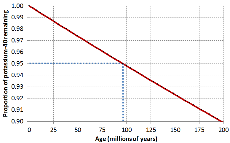
K-Ar is just one of many isotope-pairs that are useful for dating geological materials. Some of the other important pairs are listed in Table 19.2, along with the age ranges that they apply to and some comments on their applications. When radiometric techniques are applied to metamorphic rocks, the results normally tell us the date of metamorphism, not the date when the parent rock formed.
| Isotope System | Half-Life | Useful Range | Comments |
| Potassium-argon | 1.3 Ga | 10 Ka – 4.57 Ga | Widely applicable because most rocks have some potassium |
| Uranium-lead | 4.5 Ga | 1 Ma – 4.57 Ga | The rock must have uranium-bearing minerals |
| Rubidium-strontium | 47 Ga | 10 Ma – 4.57 Ga | Less precision than other methods at old dates |
| Carbon-nitrogen (a.k.a. radiocarbon dating) | 5,730 a | 100 a to 60,000 a | Sample must contain wood, bone, or carbonate minerals; can be applied to young sediments |
Table 19.2 A few of the isotope systems that are widely used for dating geological materials
Radiocarbon dating (using 14C) can be applied to many geological materials, including sediments and sedimentary rocks, but the materials in question must be younger than 60 ka. Fragments of wood incorporated into young sediments are good candidates for carbon dating, and this technique has been used widely in studies involving late Pleistocene glaciers and glacial sediments. An example is shown in Figure 19.17; radiocarbon dates from wood fragments in glacial sediments have been used to estimate the time of the last glacial advance along the Strait of Georgia.
![Figure 8.16 Radiocarbon dates on wood fragments in glacial sediments in the Strait of Georgia [SE after Clague, J, 1976, Quadra Sand and its relation to late Wisconsin glaciation of southeast British Columbia, Can. J. Earth Sciences, V. 13, p. 803-815]](https://openpress.usask.ca/app/uploads/sites/29/2017/05/Radiocarbon.png "Chapter 1. Introduction to Geology")
19.5 Other Dating Methods
There are numerous other techniques for dating geological materials, but we will examine just two of them here: tree-ring dating (i.e., dendrochronology) and dating based on the record of reversals of Earth’s magnetic field.
Dendrochronology can be applied to dating very young geological materials based on reference records of tree-ring growth going back many millennia. The longest such records can take us back over 25 ka, to the height of the last glaciation. One of the advantages of dendrochronology is that, providing reliable reference records are available, the technique can be used to date events to the nearest year.
Dendrochronology has been used to date the last major subduction zone earthquake on the coast of B.C., Washington, and Oregon. When large earthquakes strike in this setting, there is a tendency for some coastal areas to subside by one or two metres. Seawater then rushes in, flooding coastal flats and killing trees and other vegetation within a few months. There are at least four locations along the coast of Washington that have such dead trees (and probably many more in other areas). Wood samples from these trees have been studied and the ring patterns have been compared with patterns from old living trees in the region (Figure 19.18).
![Figure 8.17 Example of tree-ring dating of dead trees [SE]](https://openpress.usask.ca/app/uploads/sites/29/2017/05/tree-ring-dating.png "Chapter 1. Introduction to Geology")
![Figure 8.18 Sites in Washington where dead trees are present in coastal flats. The outermost wood of eight trees was dated using dendrochronology, and of these, seven died during the year 1699, suggesting that the land was inundated by water at that time. [SE from data in Yamaguchi, D.K., B.F. Atwater, D.E. Bunker, B.E. Benson, and M.S. Reid. 1997. Tree-ring dating the 1700 Cascadia earthquake. Nature, Vol. 389, pp. 922 - 923, 30 October 1997.]](https://openpress.usask.ca/app/uploads/sites/29/2017/05/Washington.png "Chapter 1. Introduction to Geology")
Changes in Earth’s magnetic field can also be used to date events in geologic history. The magnetic field makes compasses point toward the North Pole, but, as we’ll see in Chapter 10, this hasn’t always been the case. At various times in the past, Earth’s magnetic field has reversed itself completely, and during those times a compass would have pointed to the South Pole. By studying magnetism in volcanic rocks that have been dated isotopically, geologists have been able to delineate the chronology of magnetic field reversals going back for some 250 Ma. About 5 Ma of this record is shown in Figure 19.20, where the black bands represent periods of normal magnetism (“normal” meaning similar to the current magnetic field) and the white bands represent periods of reversed magnetism. These periods of consistent magnetic polarity are given names to make them easier to reference. The current normal magnetic field, known as Brunhes, has lasted for the past 780,000 years. Prior to that there was a short reversed period and then a short normal period known as Jaramillo.
![Figure 8.19 The last 5 Ma of magnetic field reversals. [SE after U.S. Geological Survey, http://upload.wikimedia.org/wikipedia/commons/1/13/Geomagnetic_polarity_late_Cenozoic.svg.]](https://openpress.usask.ca/app/uploads/sites/29/2017/05/magnetic-field-reversals.png "Chapter 1. Introduction to Geology")
Oceanic crust becomes magnetized by the magnetic field that exists as the crust forms from magma. As it cools, tiny crystals of magnetite that form within the magma become aligned with the existing magnetic field and then remain that way after all of the rock has hardened, as shown in Figure 19.21. Crust that is forming today is being magnetized in a “normal” sense, but crust that formed 780,000 to 900,000 years ago, in the interval between the Brunhes and Jaramillo normal periods, was magnetized in the “reversed” sense.
Chapter 3 has a discussion of Earth’s magnetic field, including where and how it is generated and why its polarity changes periodically.
![Figure 8.20 Depiction of the formation of magnetized oceanic crust at a spreading ridge. Coloured bars represent periods of normal magnetism, and the small capital letters denote the Brunhes, Jaramillio, Olduvai, and Gauss normal magnetic periods (see Figure 8.15). [SE]](https://openpress.usask.ca/app/uploads/sites/29/2017/05/magnetized-oceanic-crust.png "Chapter 1. Introduction to Geology")
Magnetic chronology can be used as a dating technique because we can measure the magnetic field of rocks using a magnetometer in a lab, or of entire regions by towing a magnetometer behind a ship or an airplane. For example, the Juan de Fuca Plate, which lies off of the west coast of B.C., Washington, and Oregon, is being and has been formed along the Juan de Fuca spreading ridge (Figure 19.22). The parts of the plate that are still close to the ridge have normal magnetism, while parts that are farther away (and formed much earlier) have either normal or reversed magnetism, depending on when the rock formed. By carefully matching the sea-floor magnetic stripes with the known magnetic chronology, we can determine the age at any point on the plate. We can see, for example, that the oldest part of the Juan de Fuca Plate that has not subducted (off the coast of Oregon) is just over 8 million years old, while the part that is subducting underneath Vancouver Island is between 0 and about 6 million years old.
![Figure 8.21 The pattern of magnetism within the area of the Juan de Fuca Plate, off the west coast of North America. The coloured shapes represent parts of the sea floor that have normal magnetism, and the magnetic time scale is shown using the same colours. The blue bands represent Brunhes, Jaramillo, and Olduvai, the green represents Gauss, and so on. (Note that, in this diagram, sea-floor magnetism is only shown for the Juan de Fuca Plate, although similar patterns exist on the Pacific Plate.) [SE]](https://openpress.usask.ca/app/uploads/sites/29/2017/05/pattern-of-magnetism.png "Chapter 1. Introduction to Geology")
Exercise 19.4 Magnetic Dating
The fact that magnetic intervals can only be either normal or reversed places significant limits on the applicability of magnetic dating. If we find a rock with normal magnetism, we can’t know which normal magnetic interval it represents, unless we have some other information.
Using Figure 19.20 for reference, determine the age of a rock with normal magnetism that has been found to be between 1.5 and 2.0 Ma based on fossil evidence.
How about a rock that is limited to 2.6 to 3.2 Ma by fossils and has reversed magnetism?
19.6 Understanding Geological Time
It’s one thing to know the facts about geological time — how long it is, how we measure it, how we divide it up, and what we call the various periods and epochs — but it is quite another to really understand geological time. The problem is that our lives are short and our memories are even shorter. Our experiences span only a few decades, so we really don’t have a way of knowing what 11,700 years means. What’s more, it’s hard for us to understand how 11,700 years differs from 65.5 Ma, or even from 1.8 Ga. It’s not that we can’t comprehend what the numbers mean — we can all get that figured out with a bit of practice — but even if we do know the numerical meaning of 65.5 Ma, we can’t really appreciate how long ago it was.
You may be wondering why it’s so important to really “understand” geological time. There are some very good reasons. One is so that we can fully understand how geological processes that seem impossibly slow can produce anything of consequence. For example, we are familiar with the concept of driving from one major city to another: a journey of several hours at around 100 km/h. Continents move toward each other at rates of a fraction of a millimetre per day, or something in the order of 0.00000001 km/h, and yet, at this impossibly slow rate (try walking at that speed!), they can move thousands of kilometres. Sediments typically accumulate at even slower rates — less than a millimetre per year — but still they are thick enough to be thrust up into monumental mountains and carved into breathtaking canyons.
Another reason is that for our survival on this planet, we need to understand issues like extinction of endangered species and anthropogenic (human-caused) climate change. Some people, who don’t understand geological time, are quick to say that the climate has changed in the past, and that what is happening now is no different. And it certainly has changed in the past. For example, from the Eocene (50 Ma) to the present day, Earth’s climate cooled by about 12°C. That’s a huge change that ranks up there with many of the important climate changes of the distant past, and yet the rate of change over that time was only 0.000024°C/century. Anthropogenic climate change has been 1.1°C over the past 100 years,[footnote]Climate change data from NASA Goddard Institute for Space Studies: http://data.giss.nasa.gov/gistemp/tabledata_v3/GLB.Ts.txt[/footnote] and that is 45,800 times faster than the rate of natural climate change since the Eocene!
One way to wrap your mind around geological time is to put it into the perspective of single year, because we all know how long it is from one birthday to the next. At that rate, each hour of the year is equivalent to approximately 500,000 years, and each day is equivalent to 12.5 million years.
Recall from Chapter 1 that if all of geological time is compressed down to a single year, Earth formed on January 1, and the first life forms evolved in late March (~3,500 Ma). The first large life forms appeared on November 13 (~600 Ma), plants appeared on land around November 24, and amphibians on December 3. Reptiles evolved from amphibians during the first week of December and dinosaurs and early mammals evolved from reptiles by December 13, but the dinosaurs, which survived for 160 million years, were gone by Boxing Day (December 26). The Pleistocene Glaciation got started at around 6:30 p.m. on New Year’s Eve, and the last glacial ice left southern Canada by 11:59 p.m.
It’s worth repeating: on this time scale, the earliest ancestors of the animals and plants with which we are familiar did not appear on Earth until mid-November, the dinosaurs disappeared after Christmas, and most of Canada was periodically locked in ice from 6:30 to 11:59 p.m. on New Year’s Eve. As for people, the first to inhabit B.C. got here about one minute before midnight, and the first Europeans arrived about two seconds before midnight.
It is common for the popular press to refer to distant past events as being “prehistoric.” For example, dinosaurs are reported as being “prehistoric creatures,” even by the esteemed National Geographic Society.[footnote]http://science.nationalgeographic.com/science/prehistoric-world/[/footnote] The written records of our history date back to about 6,000 years ago, so anything prior to that is considered “prehistoric.” But to call the dinosaurs prehistoric is equivalent to — and about as useful as — saying that Singapore is beyond the city limits of Kamloops! If we are going to become literate about geological time, we have to do better than calling dinosaurs, or early horses (54 Ma), or even early humans (2.8 Ma), “prehistoric.”
Exercise 19.5 What Happened on Your Birthday?
Using the “all of geological time compressed to one year” concept, determine the geological date that is equivalent to your birthday. First go here: http://mistupid.com/calendar/dayofyear.htm to find out which day of the year your birth date is. Then divide that number by 365, and multiply that number by 4,570 to determine the time (in millions since the beginning of geological time). Finally subtract that number from 4,570 to determine the date back from the present.
For example, April Fool’s Day (April 1) is day 91 of the year: 91/365 = 0.2493. 0.2493 x 4,570 = 1,139 million years from the start of time, and 4,570 – 1,193 = 3,377 Ma is the geological date.
Finally, go to the Foundation for Global Community’s “Walk through Time” website at http://www.globalcommunity.org/wtt/walk_menu/ to find out what was happening on your day. The nearest date to 3,377 Ma is 3,400 Ma. Bacteria ruled the world at 3,400 Ma, and there’s a discussion about their lifestyles.
Chapter 19 Summary
The topics covered in this chapter can be summarized as follows:
19.1 The Geological Time Scale
The work of William Smith was critical to the establishment of the first geological time scale early in the 19th century, but it wasn’t until the 20th century that geologists were able to assign reliable dates to the various time periods. The geological time scale is now maintained by the International Commission on Stratigraphy. Geological time is divided into eons, eras, periods, and epochs.
19.2 Relative Dating Methods
We can determine the relative ages of different rocks by observing and interpreting relationships among them, such as superposition, cross-cutting, and inclusions. Gaps in the geological record are represented by various types of unconformities.
19.3 Dating Rocks Using Fossils
Fossils are useful for dating rocks date back to about 600 Ma. If we know the age range of a fossil, we can date the rock, but some organisms lived for many millions of years. Index fossils represent shorter geological times, and if a rock has several different fossils with known age ranges, we can normally narrow the time during which the rock formed.
19.4 Isotopic Dating Methods
Radioactive isotopes decay at predictable and known rates, and can be used to date igneous and metamorphic rocks. Some of the more useful isotope systems are potassium-argon, rubidium-strontium, uranium-lead, and carbon-nitrogen. Radiocarbon dating can be applied to sediments and sedimentary rocks, but only if they are younger than 60 ka.
19.5 Other Dating Methods
There are many other methods for dating geological materials. Two that are widely used are dendrochronology and magnetic chronology. Dendrochronology, based on studies of tree rings, is widely applied to dating glacial events. Magnetic chronology is based on the known record of Earth’s magnetic field reversals.
19.6 Understanding Geological Time
While knowing about geological time is relatively easy, actually comprehending the significance of the vast amounts of geological time is a great challenge. To be able to solve important geological problems and critical societal challenges, like climate change, we need to really understand geological time.
Questions for Review
1. A granitic rock contains inclusions (xenoliths) of basalt. What can you say about the relative ages of the granite and the basalt?
2. Explain the differences between:
(a) a disconformity and a paraconformity
(b) a nonconformity and an angular unconformity
3. What are the features of a useful index fossil?
4. This diagram shows a geological cross-section. The granitic rock “f” at the bottom is the one that you estimated the age of in Exercise 19.3. A piece of wood from layer “d” has been sent for radiocarbon dating and the result was 0.55 14C remaining. How old is layer “d”?
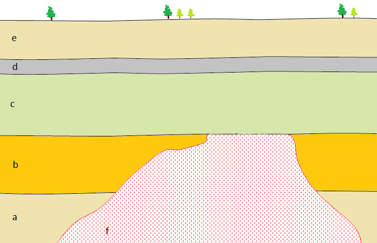
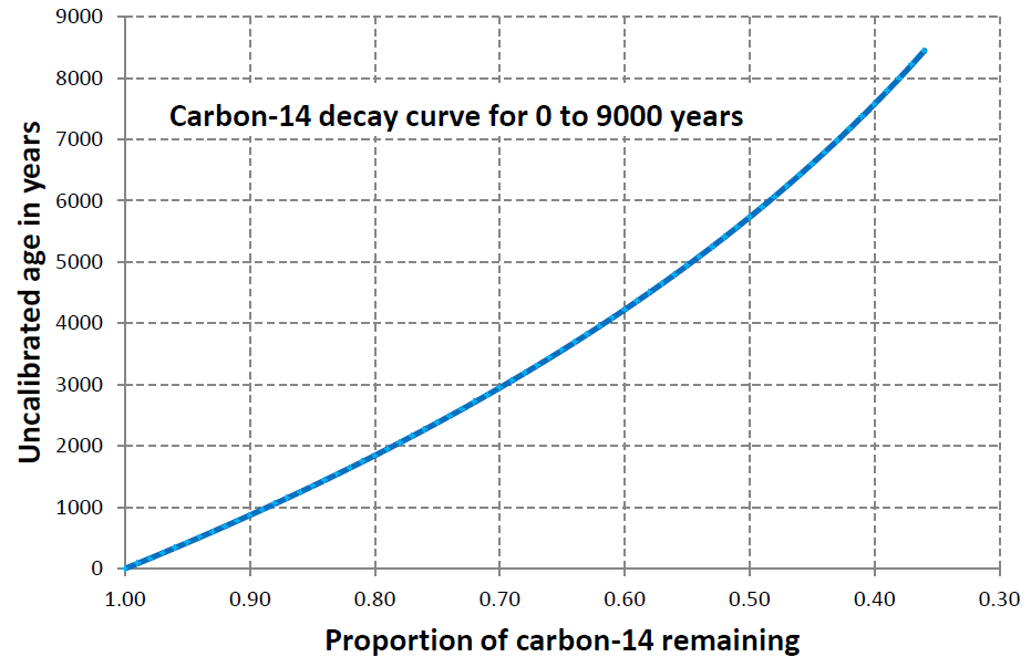
5. Based on your answer to question 4, what can you say about the age of layer “c” in the figure above?
6. What type of unconformity exists between layer “c” and rock “f”?
7. What about between layer “c” and layer “b”?
8. We can’t use magnetic chronology to date anything younger than 780,000 years. Why not?
9. How did William Smith apply the principle of faunal succession to determine the relative ages of the sedimentary rocks of England and Wales?
10. Access a copy of the geological time scale at http://www.stratigraphy.org/index.php/ics-chart-timescale. What are the names of the last age (or stage) of the Cretaceous and the first age of the Paleogene? Print out the time scale and stick it on the wall above your desk!
9.1 Clastic Sedimentary Rocks
How Clastic Sediments Become Sedimentary Rocks
Lithification is the term used to describe the process of turning sediments into solid rock. The steps in lithification are summarized in Figure 9.3.
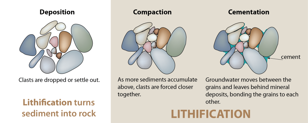
Cementation is the next step. Groundwater flowing through the pore spaces contains ions, and these ions precipitate, leaving behind minerals on the surfaces of the grains. The minerals can fill in the spaces between the grains, and accumulate where two grains are touching. Over time the minerals (called cement) bind the grains together. Quartz and calcite are common cement minerals, but depending on pressure, temperature, and chemical conditions, cement might also include other minerals such as hematite and clay.
Figure 9.4 shows sandstone viewed under a microscope. The grains are all quartz but they appear different shades of grey because they are being viewed through polarized light.[footnote]Polarized light interacts with the crystal structure in a mineral so that the light passing through the crystal will look different depending on how the crystal is oriented. If you were to rotate the slide in Figure 9.4 you would see the white grains turn black, and the black ones turn white. Different minerals respond in different ways, so this is a handy property for identifying minerals under the microscope.[/footnote] It is difficult to tell the grains from the cement in this case because both are made of quartz, but in the image on the right the more obvious grain boundaries are marked with dashed lines. Some of the cement is marked with blue shading. Using the image on the right, see if you can pick out the grain boundaries in the image in the left.
Something interesting about the sandstone in Figure 9.4 is that the cement is homoaxial. Notice the cement boundary marked by the red line in the image on the right. If you look closely you can see that it has regular steps in it. This is because the quartz in the cement has “discovered” the crystal structure of the quartz grain that it is forming around, and is continuing to build on it.
![View of sandstone under a microscope. Grains and cement are quartz. Left: Original image. Right: Visible grain boundaries are marked with dashed lines, and some of the cement is marked with blue shading. The red line shows where the cement has begun form following the crystal habit of quartz. [Karla Panchuk CC-BY 4.0 modified after Woudloper, Public Domain http://bit.ly/218II28]](https://openpress.usask.ca/app/uploads/sites/29/2017/05/sandstone_micro-1.png "Chapter 1. Introduction to Geology")
Types of Clastic Sedimentary Rocks
Clastic sedimentary rocks are named according to the characteristics of clasts (rock and mineral fragments) that make them up. Those characteristics include grain size, shape, and sorting. (To review grain sizes and the names for particles of different sizes, see Table 8.1. To review grain shape and sorting, see Figure 8.16.) The different types of clastic sedimentary rocks are summarized in Figure 9.5.
![Types of clastic sedimentary rocks. [Karla Panchuk CC-BY-NC, photos by R. Weller/ Cochise College (permission for non-commercial educational use) unless otherwise indicated]](https://openpress.usask.ca/app/uploads/sites/29/2017/05/clastic-rx-804x1024.png "Chapter 1. Introduction to Geology")
Coarse-Grained Clastic Rocks Are Conglomerate or Breccia
Clastic sedimentary rocks in which a significant proportion of the clasts are larger than 2 mm are known as conglomerate if the clasts are well rounded, and breccia if they are angular (top row of Figure 9.5). Conglomerates form in high-energy environments, such as fast-flowing rivers, where the particles can become rounded as they bump into each other while being carried along. Breccias typically form where the particles are not transported a significant distance in water, such as alluvial fans and talus slopes.
Medium-Grained Clastic Rocks Are Sandstone
Sandstone (middle row of Figure 9.5) is a very common sedimentary rock, and there are many different kinds of sandstone. It’s worth knowing something about the different types because they are organized according to characteristics that are useful for the detective work of figuring out what conditions led to the formation of a particular sandstone. Broadly, sandstones can be divided into two groups: arenite and wacke (rhymes with tacky).
Arenite is “clean” sandstone consisting mostly of sand-sized grains and cement, with less than 15% of fine-grained silt and clay in the matrix (the material between the sand-sized grains). Arenites are subdivided according to what the sand-sized grains are made of (Figure 9.6). If 90% or more of the grains are quartz, then the sandstone is a quartz arenite (also called a quartz sandstone). If more than 10% of the grains are feldspar and more of the grains are feldspar than fragments of other rocks (lithic[footnote]“Lithic” means “rock.” Lithic clasts are rock fragments, as opposed to mineral fragments.[/footnote] fragments) then the rock suffers from a surplus of names. It can be called feldspathic arenite, arkosic arenite, or just arkose. If the rock has more than 10% rock fragments, and more rock fragments than feldspar, it is lithic arenite.
![A compositional triangle for arenite sandstones, with the three most common components of sand-sized grains: quartz, feldspar, and rock fragments. Arenites have less than 15% silt or clay. [SE]](https://openpress.usask.ca/app/uploads/sites/29/2017/05/arenite-sandstones.png "Chapter 1. Introduction to Geology")
Figure 9.7 shows thin sections[footnote]Thin sections are slivers of rock sliced thinly enough that light can pass through them, and they can be examined under a microscope.[/footnote] (microscopic views) of quartz arenite, arkose, and lithic wacke. In the images, quartz grains are marked Q, feldspar grains are marked F, and lithic fragments are marked L. Notice the relative abundances of each component in the three types of rocks.
![Photos of thin sections of three types of sandstone. Some of the minerals are labelled: Q=quartz, F=feldspar and L= lithic (rock fragments). The quartz arenite and arkose have relatively little silt-clay matrix, while the lithic wacke has abundant matrix. [SE]](https://openpress.usask.ca/app/uploads/sites/29/2017/05/sandstone.png "Chapter 1. Introduction to Geology")
Fine-Grained Clastic Rocks Are Mudrocks
Rock composed of at least 75% silt- and clay-sized fragments is called mudrock. If a mudrock shows evidence of fine layers (laminations) it is called shale, otherwise it is siltstone, mudstone, or claystone, in order of increasing abundance of clay-sized particles. The fine-grained nature of mudrocks tells us that they form in very low energy environments, such as lakes, river backwaters, and the deep ocean.
Exercise 9.1 Classifying Sandstones
The images below are magnified thin sections of sandstones. Using Figures 9.5 and 9.6, give the appropriate name for each rock.
Clastic sediments are deposited in a wide range of environments, including glaciers, slope failures, rivers both fast and slow, lakes, deltas, and ocean environments both shallow and deep. Depending on the grain size in particular, they may eventually form into rocks ranging from fine mudstone to coarse breccia and conglomerate. By examining clastic sedimentary rocks for key features it is possible to translate the classification you’ve just learned into an interpretation of the environment in which the rocks were deposited.
Sediment Maturity
Maturity in sediments refers to the extent to which sediment characteristics reflect prolonged transport and weathering. Prolonged weathering and transport cause clasts to become smaller, rounder, and better sorted. It removes minerals which are more susceptible to weathering, such as feldspar and clay, leaving a sediment consisting predominantly of quartz. On the spectrum of sediment maturity, quartz sandstone would be a mature sedimentary rock, and wacke would be an immature one.
9.2 Chemical and Biochemical Sedimentary Rocks
Clastic sedimentary rocks are dominated by components that have been transported as solid clasts (clay, silt, sand, etc.). In contrast, chemical and biochemical sedimentary rocks are dominated by components that have been transported as ions in solution (e.g., Na+, Ca2+, HCO3–, etc.). There is some overlap between the two because almost all clastic sedimentary rocks contain cement formed from dissolved ions, and many chemical sedimentary rocks include some clasts. The difference between chemical and biochemical sedimentary rocks is that in biochemical sedimentary rocks, organisms play a role in turning the ions into sediment. That means the presence and nature of biochemical sedimentary rocks are linked to the life requirements of the organisms that make them. In chemical sedimentary rocks, the process is inorganic, often resulting from a body of water evaporating and concentrating the ions. It is possible for one type of sedimentary rock to form from both chemical (inorganic) and biochemical (organically mediated) processes.
Chemical and biochemical sedimentary rocks are classified based on the minerals they contain, and they are frequently dominated by a single mineral. It’s true that some clastic sedimentary rocks, such as quartz sandstone, can also be dominated by a single mineral, but the reasons are different. A clastic sedimentary rock can have whatever minerals are in the parent rock. The minerals it ends up with will depend on how much “processing” the sediments undergo by physical and chemical weathering process, and transport before the rock was cemented. Chemical and biochemical sedimentary rocks are limited largely to those minerals which dissolve relatively easily in water. Because mineral content is a defining characteristic of chemical and biochemical sedimentary rocks, we will use it to organize out discussion of these rocks.
Carbonate Rocks
Carbonate rocks are those where the dominant mineral contains the carbonate anion (CO32-). The main carbonate minerals are calcite and aragonite. Both minerals have the formula CaCO3 but they have different crystal structures. A less common carbonate mineral which is still important for forming carbonate rocks is dolomite, which has the formula CaMg(CO3)2. It is like calcite and aragonite, except that some of the calcium is replaced with magnesium.
Limestone
Limestone is made of calcite and aragonite. It can occur as a chemical sedimentary rock, forming inorganically due to precipitation, but most limestone is biochemical. In fact, limestone is by far the most common biochemical sedimentary rock.
Almost all limestone forms in marine[footnote]We use the word marine when referring to salt water (i.e., oceanic) environments, and the word aquatic when referring to freshwater environments.[/footnote] environments, and most of that forms on the shallow continental shelves[footnote]Today these are relatively narrow zones along the margins of continents, but for large parts of geologic history sea-level was much higher, and large parts of the interiors of continents were flooded.[/footnote], especially in tropical regions with coral reefs. Reefs are highly productive ecosystems populated by a wide range of organisms, many of which use calcium and bicarbonate ions in seawater to make carbonate minerals (especially calcite) for their shells and other structures. These include corals as well as green and red algae, urchins, sponges, molluscs, and crustaceans. Some of the organisms use CaCO3 to build tiny tests (shells) which accumulate on the ocean floor, but erosion also breaks them apart, scattering fragments in the surrounding region (Figure 9.8).
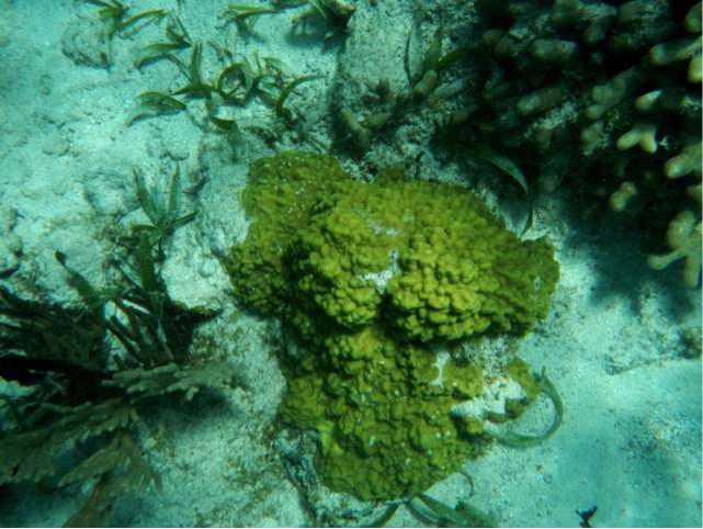
Figure 9.9 shows a cross-section through a typical reef in a tropical environment (normally between 40° N and 40° S). Reefs tend to form near the edges of steep drop-offs because the reef organisms thrive on nutrient-rich upwelling currents. As the reef builds up, it is eroded by waves and currents to produce carbonate sediments that are transported into the steep offshore fore-reef area and the shallower inshore back-reef area. These sediments are dominated by reef-type carbonate fragments of all sizes, including mud.
![Cross-section through a typical tropical reef. [SE]](https://openpress.usask.ca/app/uploads/sites/29/2017/05/tropical-reef.png "Chapter 1. Introduction to Geology")
![Carbonate rocks and sediments: (a) mollusc-rich limestone formed in a lagoon area at Ambergris, Belize, (b) foraminifera-rich sediment from a submerged carbonate sandbar near to Ambergris, Belize (c) ooids from a beach at Joulters Cay, Bahamas. [SE]](https://openpress.usask.ca/app/uploads/sites/29/2017/05/Screen-Shot-2015-06-10-at-7.09.27-PM.png "Chapter 1. Introduction to Geology")
Tufa and Travertine
Calcite can form chemical sedimentary rocks on land in a number of environments. Tufa forms at springs. The tufa towers in Figure 9.11 formed where spring water encountered lake water.
![Tufa towers (calcium carbonate) in Mono Lake, California. Evaporation keeps the concentration of ions in the lake very high, allowing the calcium carbonate to precipitate. [Brocken Inaglory CC-BY-SA http://bit.ly/20JnS7A]](https://openpress.usask.ca/app/uploads/sites/29/2017/05/1599px-Mono_lake_tufa.jpg "Chapter 1. Introduction to Geology")
![Speleothems in Cave Nefza in Tunisia [Badreddine Besbes CC-BY-SA http://bit.ly/1TqMphg]](https://openpress.usask.ca/app/uploads/sites/29/2017/05/Stalagmite_stalactite_de_grotte_de_NEFZA.jpg "Chapter 1. Introduction to Geology")
Dolostone
Dolostone (also referred to as dolomite) is the carbonate rock made of the mineral dolomite (CaMg(CO3)2). Dolostone is quite common (there’s a whole Italian mountain range named after it), which is surprising because marine organisms don’t make dolomite. All of the dolomite found in ancient rocks has been formed through magnesium replacing some of the calcium in calcite such as that contained within limestone. This process is known as dolomitization, and it is thought to involve chemical reactions with magnesium-rich water percolating through rocks and sediments containing calcite.
Chert
Chert is made of silica (SiO2). It has the same chemical formula as quartz, but is cryptocrystalline, meaning that quartz crystals are so small it is difficult to see them even under a microscope. Chert can be a chemical sedimentary rock, often forming as beds within limestone (Figure 9.13) or as irregular lenses or blobs (nodules). It can also be biochemical. Some tiny marine organisms (such as diatoms and radiolaria) make their tests from silica. When they die their tiny shells (or tests) settle slowly to the bottom where they accumulate as chert. It is possible that some of the silica in chert nodules was derived by dissolving silica tests then reprecipitating the silica.
![Chert (brown layers) interbedded with Triassic Quatsino Fm. limestone on Quadra Island, B.C. All of the layers have been folded, and the chert, being insoluble and harder than limestone, stands out. [SE]](https://openpress.usask.ca/app/uploads/sites/29/2017/05/Chert.png "Chapter 1. Introduction to Geology")
Banded Iron Formations (BIFs)
Some ancient chert beds — most dating to between 1800 and 2400 Ma — are also part of a rock known as a banded iron formation (BIF). It is a deep sea-floor deposit of iron oxide that is a common ore of iron. These rocks are called banded because they consist of alternating layers of dark iron oxide minerals (magnetite and hematite) and chert stained red by hematite (Figure 9.14).

Evaporites
In arid regions, lakes and inland seas typically have no stream outlet, and the water that flows into them is removed only by evaporation. Under these conditions, the water becomes increasingly concentrated with dissolved salts, and eventually some of these salts reach saturation levels and start to crystallize (Figure 9.15).
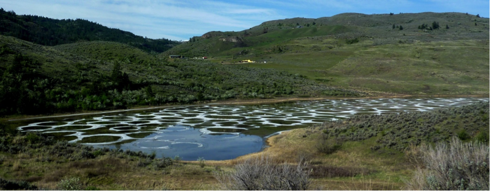
Although all evaporite deposits are unique because of differences in the chemistry of the water, in most cases minor amounts of carbonates start to precipitate when the solution is reduced to about 50% of its original volume. Gypsum (CaSO4·H2O) precipitates at about 20% of the original volume and halite (NaCl) precipitates at 10%. Other important evaporite minerals include sylvite (KCl) and borax (Na2B4O7·10H2O). Sylvite is mined as potash at numerous locations across Saskatchewan (Figure 9.16) from evaporites that formed during the Devonian (~385 Ma) when an inland sea occupied much of the region.

Exercise 9.2 Making Evaporite
This is an easy experiment that you can do at home. Pour about 50 mL (just less than 1/4 cup) of very hot water into a cup and add 2 teaspoons (10 mL) of salt. Stir until all or almost all of the salt has dissolved, then pour the salty water (leaving any undissolved salt behind) into a shallow wide dish or a small plate. Leave it to evaporate for a few days and observe the result.
It may look a little like the photo here. These crystals are up to about 3 mm across.
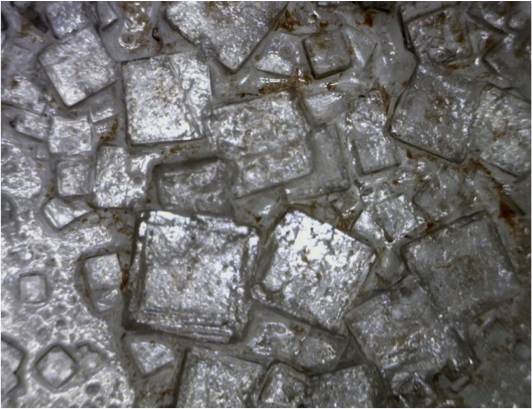
Attributions
Figure 9.10c: JoultersCayOoids By Wilson44691 under Public domain.
9.3 Organic Sedimentary Rocks
Organic sedimentary rocks are those containing large quantities of organic molecules. Organic molecules contain carbon, but in this context we are referring specifically to molecules with carbon-hydrogen bonds, such as materials from the soft tissues of plants and animals. In other words, the carbon in calcite- CaCO3 wouldn’t make calcite an organic mineral because it isn’t bonded to hydrogen.
An important organic sedimentary rock is coal. Most coal forms on swampy land adjacent to rivers and deltas, and where climates are humid and tropical to temperate. The vigorous growth of vegetation leads to an abundance of organic matter that accumulates within stagnant, acidic water. This limits decay and oxidation of the organic material. If this situation- where the dead organic matter is submerged in oxygen-poor water- is maintained for centuries to millennia, a thick layer of material can accumulate. Limited decay will transform this layer into peat (Figure 9.17a, Figure 9.18 upper left).
![Formation of coal: (a) accumulation of organic matter within a swampy area; (b) the organic matter is covered and compressed by deposition of a new layer of clastic sediments; (c) with greater burial, lignite coal forms; and (d) at even greater depths, bituminous and eventually anthracite coal form. [SE]](https://openpress.usask.ca/app/uploads/sites/29/2017/05/Formation-of-coal.png "Chapter 1. Introduction to Geology")
The further the process goes, the more the coal will go from having obvious pieces of plant material within it, to being a black, shiny mass. Low-grade lignite coal forms at depths between a few 100 m and 1,500 m and temperatures up to about 50°C (Figure 9.17c). This is still a relatively early stage in the coal formation process, so the lignite can resemble plant material very closely (Figure 9.18 upper right).
At between 1,000 m to 5,000 m depth and temperatures up to 150°C m, bituminous coal forms (Figure 9.17d, 9.18 lower right). At depths beyond 5,000 m and temperatures over 150°C, anthracite coal forms (Figure 9.18 lower left). In fact, as temperatures rise, the lower-grade forms of coal are actually being transformed from sedimentary to metamorphic rocks.
![The formation of coal begins when plant matter is prevented from decaying by accumulating in low-oxygen, acidic water. A layer of peat forms. Heating and compression of peat form lignite, bituminous coal, and then anthracite, as pressures and temperatures increase. [KP]](https://openpress.usask.ca/app/uploads/sites/29/2017/05/coal.png "Chapter 1. Introduction to Geology")
9.4 Depositional Environments and Sedimentary Basins
Sediments accumulate in a wide variety of environments, both on the continents and in the oceans. Some of the more important of these environments are illustrated in Figure 9.19.
![Some of the important depositional environments for sediments and sedimentary rocks [SE after Mike Norton CC-BY-SA http://bit.ly/1QpPcIw]](https://openpress.usask.ca/app/uploads/sites/29/2017/05/sediments.png "Chapter 1. Introduction to Geology")


Most of the sediments that you might see around you, including talus on steep slopes, sand bars in streams, or gravel in road cuts, will never become sedimentary rocks because they have only been deposited relatively recently — perhaps a few centuries or millennia ago — and will be re-eroded before they are buried deep enough beneath other sediments to be lithified. In order for sediments to be preserved long enough to be turned into rock- a process that takes millions or tens of millions of years- they need to have been deposited in a basin that will last that long. Most such basins are formed by plate tectonic processes, and some of the more important examples are shown in Figure 9.20.
![Some of the more important types of tectonically produced basins: (a) trench basin, (b) forearc basin, (c) foreland basin, and (d) rift basin [SE]](https://openpress.usask.ca/app/uploads/sites/29/2017/05/basins.png "Chapter 1. Introduction to Geology")
A forearc basin lies between the subduction zone and the volcanic arc, and may be formed in part by friction between the subducting plate and the overriding plate, which pulls part of the overriding plate down. The Strait of Georgia is a forearc basin.
A foreland basin is caused by the mass of the volcanic range depressing the crust on either side. Foreland basins are not only related to volcanic ranges, but can form adjacent to fold belt mountains like the Canadian Rockies. A rift basin forms where continental crust is being pulled apart, and the crust on both sides the rift subsides. As rifting continues this eventually becomes a narrow sea, and then an ocean basin. The East African rift basin represents an early stage in this process.
9.5 Sedimentary Structures and Fossils
Through careful observation over the past few centuries, geologists have discovered that the accumulation of sediments and sedimentary rocks takes place according to some important geological principles, as follows:
- The principle of original horizontality states that sediments accumulate in essentially horizontal layers. The implication is that tilted sedimentary layers observed to day must have been subjected to tectonic forces.
- The principle of superposition states that sedimentary layers are deposited in sequence, and that unless the entire sequence has been turned over by tectonic processes, the layers at the bottom are older than those at the top.
- The principle of inclusions states that any rock fragments in a sedimentary layer must be older than the layer. For example, the cobbles in a conglomerate must have been formed before the conglomerate.
- The principle of faunal succession states that there is a well-defined order in which organisms have evolved through geological time, and therefore the identification of specific fossils in a rock can be used to determine its age.
In addition to these principles that apply to all sedimentary rocks, a number of other important characteristics of sedimentary processes lead to the development of distinctive sedimentary features in specific sedimentary environments. By understanding the origins of these features, we can make some very useful inferences about the processes that led to deposition the rocks that we are studying.
Bedding, for example, is the separation of sediments into layers that either differ from one another in textures, composition, colour, or weathering characteristics, or are separated by partings — narrow gaps between adjacent beds (Figure 9.21). Bedding is an indication of changes in depositional processes that may be related to seasonal differences, changes in climate, changes in locations of rivers or deltas, or tectonic changes. Partings may represent periods of non-deposition that could range from a few decades to a few centuries. Bedding can form in almost any depositional environment.
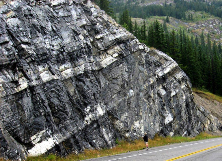
Cross-bedding is bedding that contains angled layers and forms when sediments are deposited by flowing water or wind. An example is shown in Figure 9.22. Cross-beds in streams tend to be on the scale of centimetres to tens of centimetres, while those in aeolian (wind deposited) sediments can be on the scale of metres to several metres.
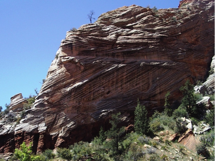
Cross-beds form as sediments are deposited on the leading edge of an advancing ripple or dune. Each layer is related to a different ripple that advances in the flow direction, and is partially eroded by the following ripple (Figure 9.23). Cross-bedding is a very important sedimentary structure to recognize because it can provide information on the direction of current flows and, when analyzed in detail, on other features like the rate of flow and the amount of sediment available.
![Formation of cross-beds as a series of ripples or dunes migrates with the flow. Each ripple advances forward (right to left in this view) as more sediment is deposited on its leading face. [SE]](https://openpress.usask.ca/app/uploads/sites/29/2017/05/Formation-of-cross-beds.png "Chapter 1. Introduction to Geology")
Graded bedding is characterized by a change in grain size from bottom to top within a single bed. “Normal” graded beds are coarse at the bottom and become finer toward the top, a product of deposition from a slowing current (Figure 9.24). Some graded beds are reversed (coarser at the top), and this normally results from deposition by a fast-moving debris flow. Most graded beds form in a submarine-fan environment (see Figure 9.19), where sediment-rich flows descend periodically from a shallow marine shelf down a slope and onto the deeper sea floor.
![Figure 9.25 Graded bedding going from pebbles at the bottom to sand at the top. [Natural Resources, Government of Newfoundland and Labrador, by permission http://bit.ly/1UdaCIC]](https://openpress.usask.ca/app/uploads/sites/29/2017/05/gradedlg-300x195.jpg "Chapter 1. Introduction to Geology")
![An illustration of imbrication of clasts in a fluvial environment. [SE]](https://openpress.usask.ca/app/uploads/sites/29/2017/05/imbrication-of-clasts.png "Chapter 1. Introduction to Geology")
![Mud cracks in a tidal flat area in England [Alan Parkinson CC-BY-SA http://bit.ly/1KwF3HK]](https://openpress.usask.ca/app/uploads/sites/29/2017/05/Mud-cracks.png "Chapter 1. Introduction to Geology")
A Note About Fossils
Fossils are not covered in detail in this book, but they are extremely important for understanding sedimentary rocks. Fossils can be used to date sedimentary rocks, but just as importantly, they tell us a great deal about the depositional environment of the sediments and the climate at the time. For example, they can help to differentiate marine, aquatic, and terrestrial environments; estimate the depth of the water; detect the existence of currents; and estimate average temperature and precipitation.
The tests of tiny marine organisms (mostly foraminifera) have been recovered from deep-ocean sediment cores from all over the world, and their isotopic signatures have been measured. As we’ll see in later, this provides us with information about the changes in average global temperatures.
Exercise 9.3 Interpretation of Past Environments
Sedimentary rocks can tell us a great deal about the environmental conditions that existed during the time of their formation. For each of the following rocks, make some inferences about the following:
- source rock
- weathering
- sediment transportation (how, how far)
- depositional conditions
Quartz sandstone: no feldspar, well-sorted and well-rounded quartz grains, cross-bedding
Feldspathic sandstone and mudstone: feldspar, volcanic fragments, angular grains, repetitive graded bedding from sandstone upwards to mudstone
Conglomerate: well-rounded pebbles and cobbles of granite and basalt; imbrication
Breccia: poorly sorted, angular limestone fragments; orange-red matrix
9.6 Groups, Formations, and Members
Geologists who study sedimentary rocks need ways to divide them into manageable units, and they also need to give those units names so that they can easily be referred to and compared with other rocks deposited in other places. The International Commission on Stratigraphy (ICS) (http://www.stratigraphy.org/) has established a set of conventions for grouping, describing, and naming sedimentary rock units.
The main stratigraphic unit is a formation, which according to the ICS, should be established with the following principles in mind:
The contrast in lithology between formations required to justify their establishment varies with the complexity of the geology of a region and the detail needed for geologic mapping and to work out its geologic history. No formation is considered justifiable and useful that cannot be delineated at the scale of geologic mapping practiced in the region. The thickness of formations may range from less than a meter to several thousand meters.
In other words, a formation is a series of beds that is distinct from other beds above and below, and is thick enough to be shown on the geological maps that are widely used within the area in question. In most parts of the world, geological mapping is done at a relatively coarse scale, and so most formations are in the order of a few hundred metres thick. At that thickness, a typical formation would appear on a typical geological map as an area that is at least a few millimetres thick.
A series of formations can be classified together to define a group, which could be as much as a few thousand metres thick, and represents a series of rocks that were deposited within a single basin (or a series of related and adjacent basins) over a few million to a few tens of millions of years.
In areas where detailed geological information is needed (for example, within a mining or petroleum district) a formation might be divided into members, where each member has a specific and distinctive lithology (rock type). For example, a formation that includes both shale and sandstone might be divided into members, each of which is either shale or sandstone. In some areas, where particular detail is needed, members may be divided into beds, but this is only applicable to beds that have a special geological significance. Groups, formations, and members are typically named for the area where they are found.
The sedimentary rocks of the Nanaimo Group provide a useful example for understanding groups, formations, and members. During the latter part of the Cretaceous Period, from about 90 Ma to 65 Ma, a thick sequence of clastic rocks was deposited in a foreland basin between what is now Vancouver Island and the B.C. mainland (Figure 9.27). The Nanaimo Group strata comprise a 5000 m thick sequence of conglomerate, sandstone, and mudstone layers. Coal was mined from Nanaimo Group rocks from around 1850 to 1950 in the Nanaimo region, and is still being mined in the Campbell River area.
![The distribution of the Upper Cretaceous Nanaimo Group rocks on Vancouver Island, the Gulf Islands, and in the Vancouver area. [SE after Mustard, P., 1994, The Upper Cretaceous Nanaimo Group, Georgia Basin, in J. Monger (ed) Geology and Geological Hazards of the Vancouver Region, Geol. Survey of Canada, Bull. 481, pp. 27-95]](https://openpress.usask.ca/app/uploads/sites/29/2017/05/Upper-Cretaceous-Nanaimo-Group-rocks.png "Chapter 1. Introduction to Geology")
![The formations of the Nanaimo Group. Formations that are predominantly fine-grained are shaded. In figures like this one the layers are always listed with the oldest at the bottom and the youngest at the top. [Based on data in Mustard, P., 1994, The Upper Cretaceous Nanaimo Group, Georgia Basin, in J. Monger (ed) Geology and Geological Hazards of the Vancouver Region, Geol. Survey of Canada, Bull. 481, p. 27-95.]](https://openpress.usask.ca/app/uploads/sites/29/2017/05/Nanaimo-Group-1024x508.png "Chapter 1. Introduction to Geology")
Although there is a great deal of variety in the Nanaimo Group rocks, and it would take hundreds of photographs to illustrate all of the different types of rocks, a few representative examples are provided in Figure 9.29.
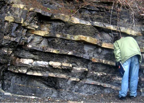


Chapter 9 Summary
The topics covered in this chapter can be summarized as follows:
9.1 Clastic Sedimentary Rocks
Sedimentary clasts are classified based on their size, and variations in clast size have important implications for transportation and deposition. Clastic sedimentary rocks range from conglomerate to mudstone. Clast size, sorting, composition, and shape are important features that allow us to differentiate clastic rocks and understand the processes that took place during their deposition.
9.2 Chemical and Biochemical Sedimentary Rocks
Chemical and biochemical sedimentary rocks form from ions that were transported in solution, and then converted into minerals by chemical and/or biological processes. The most common chemical rock, limestone, typically forms in shallow tropical marine environments, where biological activity is a very important factor. Chert and banded iron formation are deep-ocean sedimentary rocks. Evaporites form where the water of lakes and inland seas becomes supersaturated due to evaporation.
9.3 Organic Sedimentary Rocks
Organic sedimentary rocks contain abundant organic carbon molecules (molecules with carbon-hydrogen bonds). An example is coal, which forms when dead plant material is preserved in stagnant swamp water, and later compressed and heated.
9.4 Depositional Environments and Sedimentary Basins
There is a wide range of depositional environments, both on land (glaciers, lakes, rivers, etc.) and in the ocean (deltas, reefs, shelves, and the deep-ocean floor). In order to be preserved, sediments must accumulate in long-lasting sedimentary basins, most of which form through plate-tectonic processes.
9.5 Sedimentary Structures and Fossils
The deposition of sedimentary rocks takes place according to a series of important principles, including original horizontality, superposition, and faunal succession. Sedimentary rocks can also have distinctive structures that are important in determining their depositional environments. Fossils are useful for determining the age of a rock, the depositional environment, and the climate at the time of deposition.
9.6 Groups, Formations, and Members
Sedimentary sequences are classified into groups, formations, and members so that they can be referred to easily and without confusion.
Questions for Review
- What are the minimum and maximum sizes of sand grains?
- The material that makes up a rock such as conglomerate cannot be deposited by a slow-flowing river. Why not?
- Describe the two main processes of lithification.
- What is the difference between a lithic arenite and a lithic wacke?
- How does a feldspathic arenite differ from a quartz arenite?
- What can we say about the source area lithology and the weathering and transportation history of a sandstone that is primarily composed of rounded quartz grains?
- What is the original source of the carbon that is present within carbonate deposits such as limestone?
- What long-term environmental change on Earth led to the deposition of banded iron formations?
- Name two important terrestrial depositional environments and two important marine ones.
- What is the origin of a foreland basin, and how does it differ from a forearc basin?
- Explain the origin of (a) bedding, (b) cross-bedding, (c) graded bedding, and (d) mud cracks.
- Under what conditions is reverse graded bedding likely to form?
- What are the criteria for the application of a formation name to a series of sedimentary rocks?
- Explain why some of the Nanaimo Group formations have been divided into members, while others have not.